Modern cosmology uses Einstein’s theory of general relativity to connect the geometry and expansion of the universe to its matter and energy content. The first stage of this project focused on developing the theoretical background needed for cosmological research through an independent study of general relativity and physical cosmology. This work involved deriving key equations and concepts, including covariant derivatives, Christoffel symbols, geodesic motion, Einstein’s field equation, and cosmological expansion. Part of this material was presented in a mid-program presentation titled “Deriving the Einstein Field Equation: How Matter Curves Spacetime.”

The next stage involved writing MATLAB programs to reproduce cosmological figures from Principles of Physical Cosmology by P. J. E. Peebles [1]. These calculations modeled how quantities such as lookback time, angular-size distance, luminosity distance, line-of-sight intersection probabilities, and the growth of density fluctuations depend on redshift and cosmological density parameters. Many of the programs were built around the dimensionless expansion function, E(z) = H(z)/H₀, and the distance relations obtained by integrating functions of E(z).

After establishing the theoretical and computational foundation, the project shifted toward reproducing results from a published cosmology paper by Omer Farooq and Bharat Ratra. The paper uses 28 independent measurements of the Hubble parameter, H(z), between redshifts 0.07 and 2.3 to constrain cosmological parameters. The results indicate that the Hi(z) measurements favor a currently accelerating expansion of the universe at approximately three-sigma confidence [2].

Fig. 1. The 28 observed Hubble-parameter measurements used in the cosmological analysis, plotted as a function of redshift. The vertical error bars represent the reported one-sigma uncertainties, σ_H, associated with each measurement. Data compiled by Farooq and Ratra [2] from the observational sources listed in Refs. [4–10]

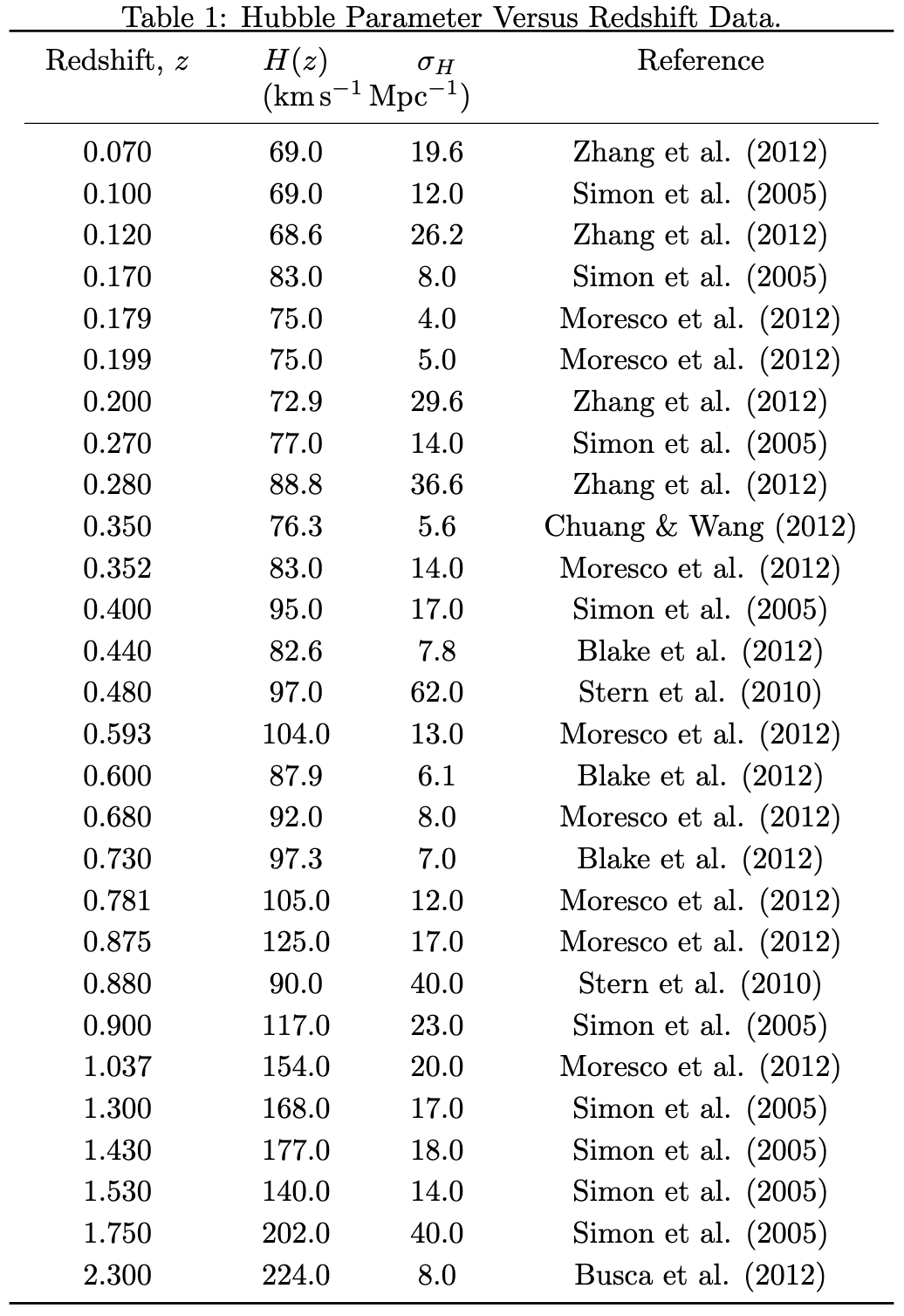
Table 1: Redshift, observed Hubble-parameter, and one-sigma uncertainty values for the 28 H(z) measurements used in the ΛCDM and XCDM analyses. Data compiled by Farooq and Ratra [2] from the observational sources listed in Refs. [4–10].

The computational analysis focused on two cosmological models. The Lambda Cold Dark Matter (ΛCDM) model describes dark energy using Einstein’s cosmological constant, Λ, and allows the present matter-density parameter, Ω_m0, and cosmological-constant density parameter, Ω_Λ, to vary. The spatially flat X-Cold Dark Matter (XCDM) model instead describes dark energy using a constant equation-of-state parameter, ω_X, while constraining the dark-energy density through spatial flatness. When ω_X = −1, XCDM reduces to the corresponding spatially flat ΛCDM model.

For both models, theoretical predictions for H(z) were compared with the observational dataset using two Gaussian prior measurements of the Hubble constant: H₀ = 68.0 ± 2.8 km s⁻¹ Mpc⁻¹ and H₀ = 73.8 ± 2.4 km s⁻¹ Mpc⁻¹.

Rather than fixing the Hubble constant at either prior mean, its uncertainty was incorporated by analytically marginalizing the likelihood over all physically allowed positive values of H₀. Figure 2 illustrates how A, B, and C are constructed from the observed H(z) measurements, their uncertainties, the model expansion function E(z), and the selected Gaussian H₀ prior. These quantities determine the marginalized chi-square evaluated for each proposed set of cosmological parameters.

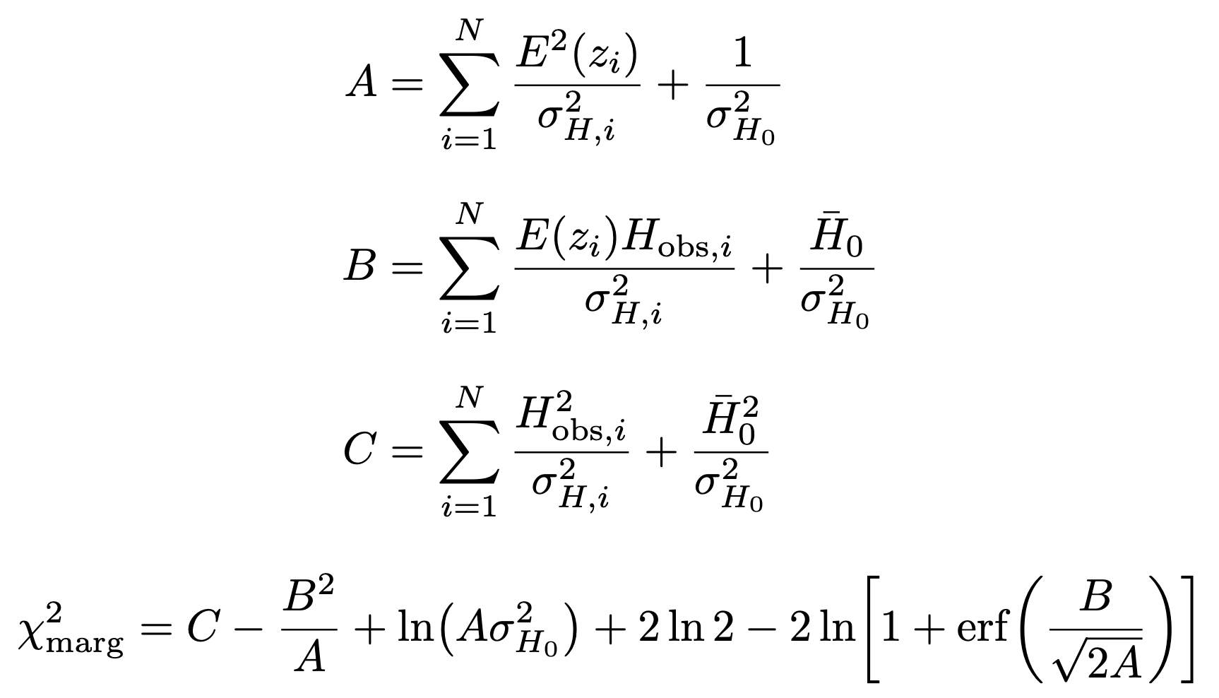
Fig. 2. Marginalization of the H(z) likelihood over the Hubble constant, H₀. Here, H̅₀ and σH₀ are the mean and standard deviation of the Gaussian H₀ prior, respectively, and erf denotes the error function.

A Python Markov chain Monte Carlo (MCMC) sampler was then developed using the emcee package. The program evaluates the marginalized likelihood, calculates best-fit parameter values and confidence intervals, and produces diagnostic information for each run. GetDist was used to convert the MCMC samples into one-, two-, and three-sigma confidence contours. Separate scripts were created for the ΛCDM and XCDM cases, allowing the same statistical framework to be applied across multiple cosmological models.

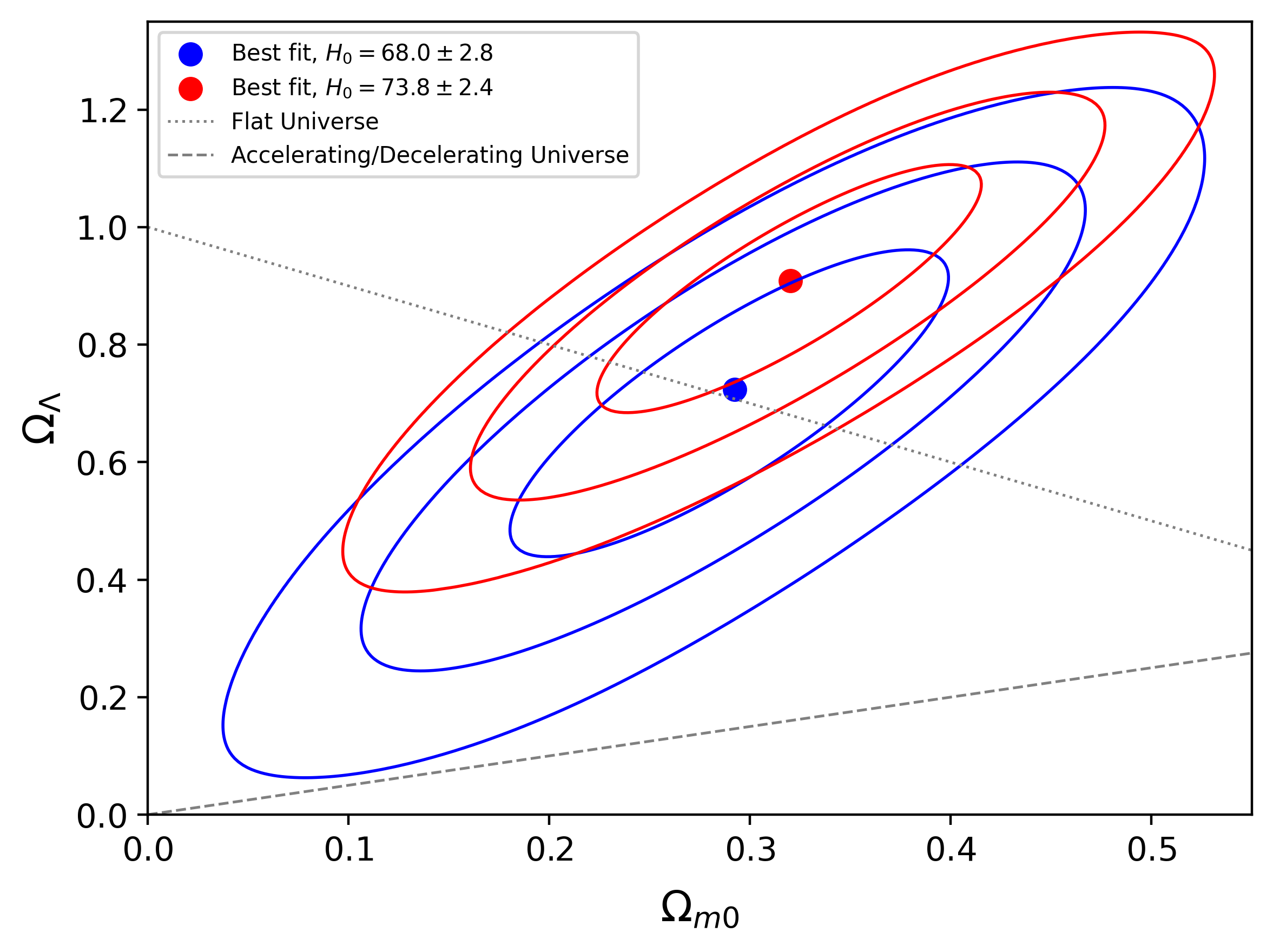
Fig 3. Combined ΛCDM constraints in the Ω_m0–Ω_Λ parameter plane. Each contour set shows the one-, two-, and three-sigma confidence regions for a different Gaussian H₀ prior. The solid circles indicate the corresponding best-fit parameter values.

Figure 3 shows the combined ΛCDM constraints in the Ω_m0–Ω_Λ plane. The confidence contours display the degeneracy between the matter and cosmological-constant density parameters and show how the preferred parameter region changes when a different H₀ prior is used. The plot also includes the spatially flat-universe condition, Ω_m0 + Ω_Λ = 1, and the boundary separating accelerating and decelerating cosmological expansion.

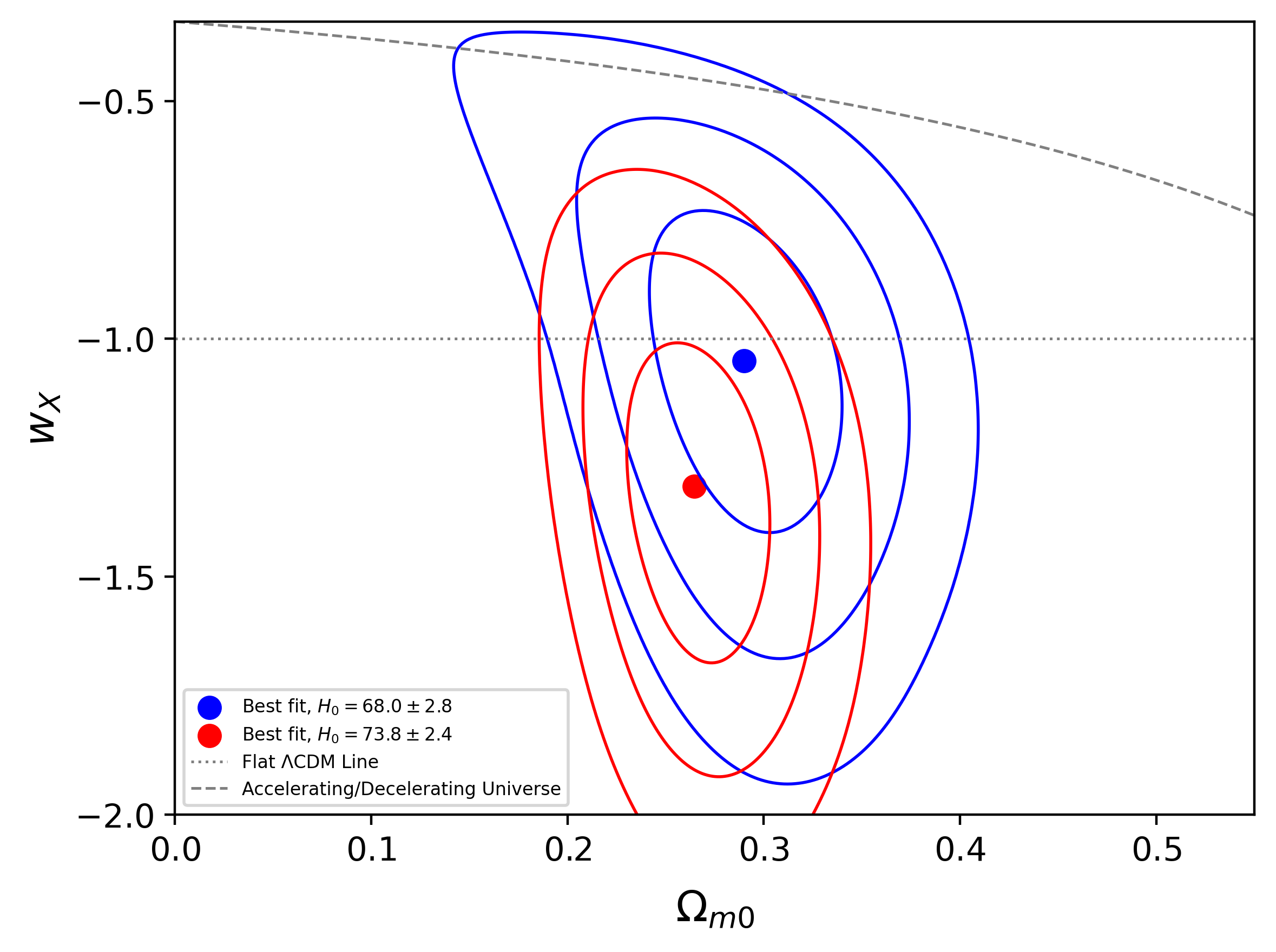
Fig.4. Combined XCDM constraints in the Ω_m0–ω_X parameter plane. Each contour set shows the one-, two-, and three-sigma confidence regions for a different Gaussian H₀ prior. The solid circles indicate the corresponding best-fit parameter values.

Figure 4 shows the corresponding XCDM constraints in the Ω_m0–ω_X plane. The line ω_X = −1 identifies the ΛCDM limit of the XCDM parametrization, while the accelerating–decelerating boundary provides a physical interpretation of the allowed parameter space. The confidence regions favor an accelerating universe, although the H(z) data permit a broader range of values for ω_X than for Ω_m0.

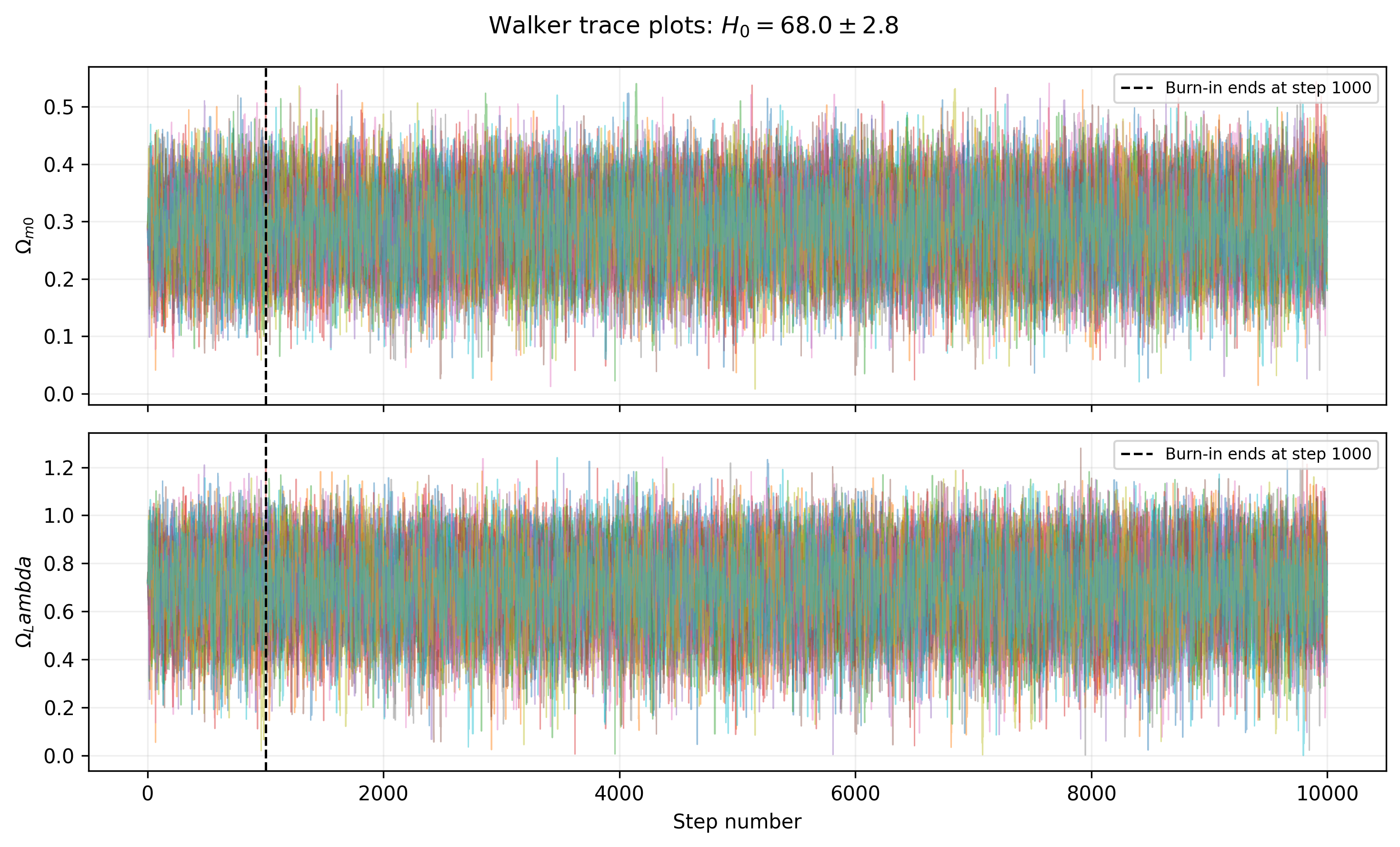
Fig. 5. MCMC walker traces for the ΛCDM model using H₀ = 68.0 ± 2.8 km s⁻¹ Mpc⁻¹. Each colored line represents a walker sampling the matter-density parameter, Ω_m0, and the cosmological-constant density parameter, Ω_Λ. The vertical dashed line marks the end of the 1,000-step burn-in period.

Figure 5 shows the MCMC walker traces for the ΛCDM case using H₀ = 68.0 ± 2.8 km s⁻¹ Mpc⁻¹. These plots provide visual convergence diagnostics by showing how the walkers explore the parameter space without sustained drift. Acceptance fractions and integrated autocorrelation times were also calculated to evaluate sampling performance and determine whether the chains were sufficiently long.

This project progressed from the mathematical foundations of general relativity to the construction of a reusable statistical tool for observational cosmology. The completed sampler combines likelihood evaluation, parameter estimation, convergence diagnostics, and confidence-contour generation within a single Python framework. The next step will be to extend this analysis to larger combinations of lower-redshift observations, including supernova, baryon acoustic oscillation, quasar, gamma-ray burst, and updated H(z) datasets [3].

References

1] Peebles, P. J. E. Principles of Physical Cosmology. Princeton University Press, 1993.

[2] Omer Farooq and Bharat Ratra, “Hubble Parameter Measurement Constraints on the Cosmological Deceleration-Acceleration Transition Redshift,” The Astrophysical Journal Letters, Vol. 766, No. 1, L7, 2013.

[3] Shulei Cao and Bharat Ratra, “H₀ = 69.8 ± 1.3 km s⁻¹ Mpc⁻¹, Ω_m0 = 0.2882 ± 0.017, and Other Constraints from Lower-Redshift, Non-CMB, Expansion Rate Data,” Physical Review D, Vol. 107, 103521, 2023.

[4] Joan Simon, Licia Verde, and Raul Jimenez, “Constraints on the Redshift Dependence of the Dark Energy Potential,” Physical Review D, Vol. 71, 123001, 2005.

[5] Daniel Stern, Raul Jimenez, Licia Verde, Marc Kamionkowski, and S. Adam Stanford, “Cosmic Chronometers: Constraining the Equation of State of Dark Energy. I: H(z) Measurements,” Journal of Cosmology and Astroparticle Physics, No. 2, 008, 2010.

[6] Michele Moresco, Andrea Cimatti, Raul Jimenez, Lucia Pozzetti, Gianni Zamorani, Matteo Bolzonella, James Dunlop, François Lamareille, Marco Mignoli, H. Pearce, and collaborators, “Improved Constraints on the Expansion Rate of the Universe up to z ∼ 1.1 from the Spectroscopic Evolution of Cosmic Chronometers,” Journal of Cosmology and Astroparticle Physics, No. 8, 006, 2012.

[7] Nicolás G. Busca, Timothée Delubac, James Rich, Stephen Bailey, Andreu Font-Ribera, David Kirkby, Jean-Marc Le Goff, Matthew M. Pieri, Anže Slosar, Éric Aubourg, and collaborators, “Baryon Acoustic Oscillations in the Lyα Forest of BOSS Quasars,” Astronomy & Astrophysics, Vol. 552, A96, 2013.

[8] Cong Zhang, Han Zhang, Shuo Yuan, Siqi Liu, Tong-Jie Zhang, and Yan-Chun Sun, “Four New Observational H(z) Data from Luminous Red Galaxies in the Sloan Digital Sky Survey Data Release Seven,” Research in Astronomy and Astrophysics, Vol. 14, pp. 1221–1233, 2014. The dataset was originally circulated as arXiv:1207.4541 in 2012.

[9] Chris Blake, Sarah Brough, Matthew Colless, Carlos Contreras, Warrick Couch, Scott Croom, Darren Croton, Tamara M. Davis, Michael J. Drinkwater, Karl Forster, and collaborators, “The WiggleZ Dark Energy Survey: Joint Measurements of the Expansion and Growth History at z < 1,” Monthly Notices of the Royal Astronomical Society, Vol. 425, pp. 405–414, 2012.

[10] Chia-Hsun Chuang and Yun Wang, “Modeling the Anisotropic Two-Point Galaxy Correlation Function on Small Scales and Improved Measurements of H(z), D_A(z), and f(z)σ₈(z) from the Sloan Digital Sky Survey DR7 Luminous Red Galaxies,” Monthly Notices of the Royal Astronomical Society, Vol. 435, pp. 255–262, 2013. The study was first submitted as arXiv:1209.0210 in 2012.

Contact

Email: rrengan511@gmail.com

LinkedIn: Ryan Renganeschi

 

Acknowledgments

I would like to thank Dr. Bharat Ratra for his mentorship, guidance, and support throughout this project. I would also like to thank Dr. Olga Avsajanishvili for her advice on the MCMC analysis and confidence-contour construction. I would like to extend my gratitude to Dr. Bret Flanders, Dr. Cosmin Blaga, and Kim Coy for organizing and supporting the Kansas State University Physics REU program, as well as to the fellow researchers in my cohort and the broader community who helped make Kansas State University feel like home throughout the summer.

This material is based upon work supported by the National Science Foundation under Grant No. 2548403. Any opinions, findings, conclusions, or recommendations expressed in this material are those of the author and do not necessarily reflect the views of the National Science Foundation.

Final Presentation