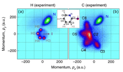
Coulomb Explosion Imaging is an experimental technique for investigating the dynamics of molecules. The first step of the technique involves stripping as many electrons as possible off of a molecule. This ionization is commonly carried out by hitting the target molecule with an intense infrared laser. With few negatively-charged electrons present, the Coulomb repulsion between the nuclei will cause the molecule to dissociate. As the pieces fly away, they are detected. Using this information, the molecule’s dynamics can be studied. For an example of this type of experimental data,

My work this summer has involved connecting theory to a specific experiment of this type, utilizing “pump-probe” techniques. In this experiment, CH2I2 was first hit with a “pump” pulse of ultraviolet light with a wavelength of 200 nanometers. This added energy raised the molecule to an excited state. Then, the typical infrared “probe” was used to perform the Coulomb Explosion. My portion of the project was theoretical; theorists generally attempt to explain or predict experimental results using computational models.

My goal was to model the potential energy curves for excited states of CH2I2, so that they could be compared to the experimental results. In particular, my goal was to characterize these potential curves to an energy of 6.199 eV–the energy of the 200 nm pump pulse. This was done using a program called Molpro. I used the Multi-Configurational Self-Consistent Field method (MCSCF) to solve the molecular Schrödinger equation, finding the minimum potential energy. The model uses the Born-Oppenheimer approximation to simplify the equation by disregarding terms describing nuclear motion. This could be thought of as assuming the nuclei do not move much, since they are much slower than the electrons.

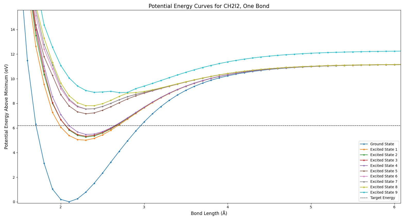
I provided the model with a molecular geometry, and it determined the best possible way to arrange the electrons. This amounted to determining the lowest possible potential energy. So, I could vary the geometry and make a potential energy curve. I first did this by varying one of the C-I bond lengths. The full view of the resulting potential curve can be seen in Fig. 2.

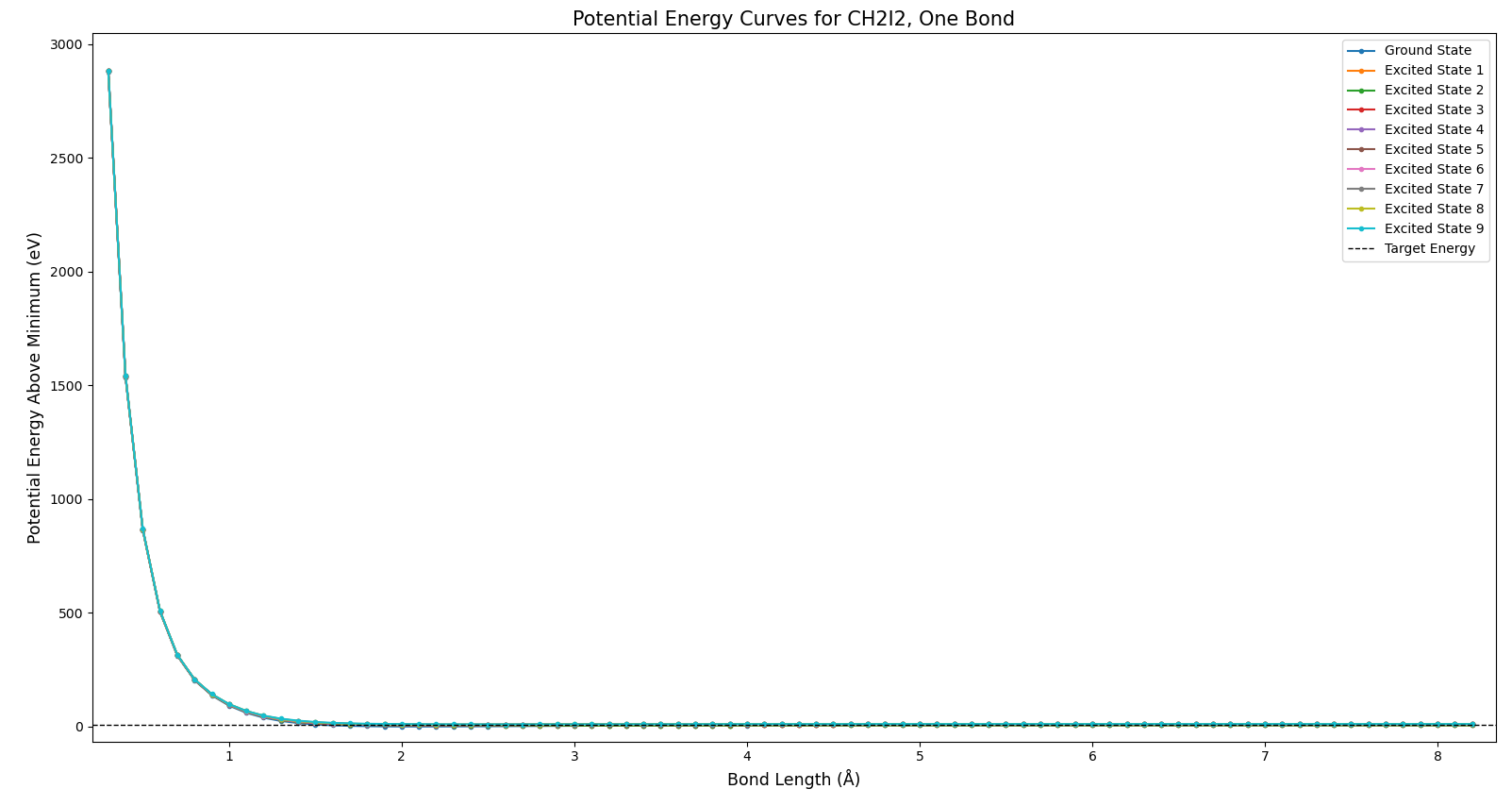
This plot is not particularly illustrative, but it does show two things. Firstly, the energies all approach infinity as the bond length goes to zero. Secondly, the energies approach constant values as the bond length approaches infinity. Both of these behaviors are expected for Coulomb potentials. At longer distances, the bond is essentially broken, and there is no more attraction. In this and all future plots, the horizontal dashed line represents the energy of a 200 nm pump photon. Now to examine some more specific portions of this plot, in Fig. 3.

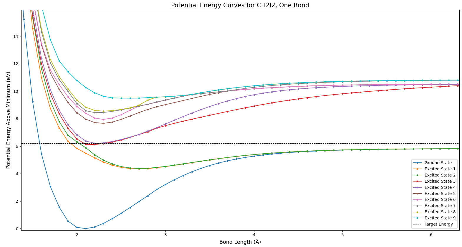
In Fig. 3 we see the ground state of the molecule, in dark blue. Interestingly, as the bond length increases and the bond is broken, the various excited states approach different levels. How can breaking a bond result in different total energies? This actually does make sense–in cases where an excited state goes to a different energy than the ground state, some of the products exist in an excited state after the bond is broken.

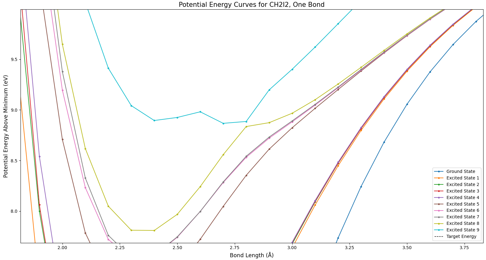
Figure 4 shows a phenomenon referred to as an avoided crossing. Note how the green and red states seem like they might cross, but suddenly move away from each other. All that this means is that there is something which prevents those states from crossing. There’s no way to tell from this plot what the cause might be; these potential curves are one-dimensional slices of very complex many-dimensional curves. Each parameter of the molecule provides another dimension–this includes bond lengths, bond angles, and the angles between bond planes.

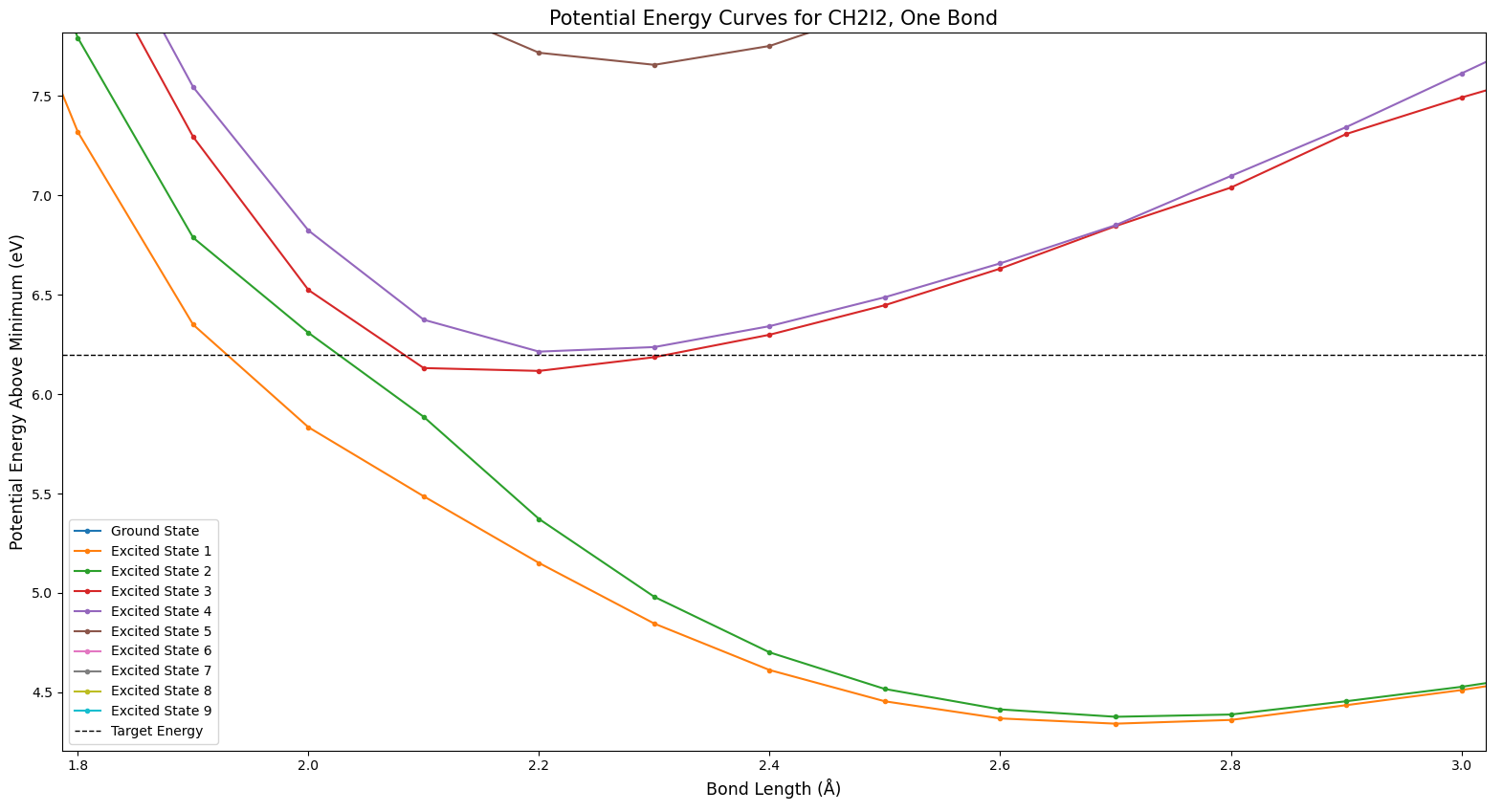
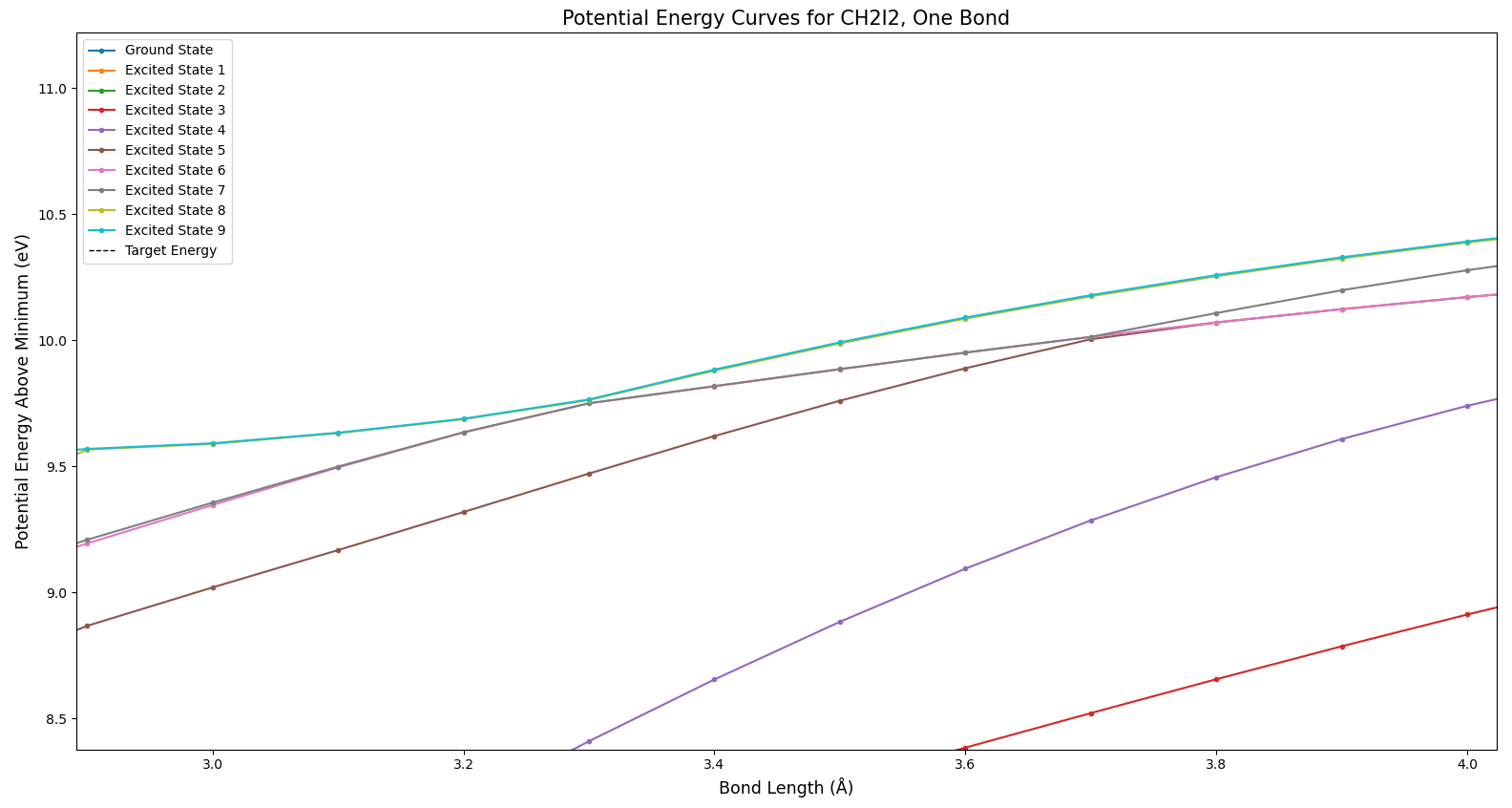
Figure 5 shows another type of phenomenon which is expected from potential surfaces like these. In this figure, the teal and gray states seem to cross, as do the gray and pink or brown states. But the colors don’t cross. The highest state is always teal, for example. Do the states cross, or not? In fact, they do. The odd coloration involved is a side effect of the way this data is formatted. Because Molpro was run on each bond length value separately, the different values effectively can’t “communicate” with each other–the lines drawn between points are just for the convenience of the viewer. It’s simply defined that the highest state is always colored teal for relative ease of viewing, and the coloring issue when states cross is an unavoidable side effect. There’s not much of a way around this with the way the data is structured; crossings like this are an expected item.

Finally, let’s zoom in on one portion of interest within the two bond curve. Figure 7 shows this portion of interest, which you may have noticed as well in Fig. 6. The teal and yellowish states show distinctly odd behavior around the center of Fig. 7. This is actually not correct; it is a result of the way Molpro operates. Molpro averages the potential energy of each state, and tries to minimize that average–these states are simply outliers, and the average is still at its minimum possible arrangement (as far as Molpro knows). This could potentially be fixed by increasing the active space which Molpro uses.

Active space refers to the number of electrons and orbitals which Molpro tries to optimize–since the molecule is large, only the relevant electrons are considered. A reduced active space cuts calculation time from four hours to four minutes. Increasing the size of the active space would be the best way to remove the erroneous portion of the two bond curve. All in all, this project’s goal was achieved–excited states of diiodomethane were characterized (and potential energy curves were drawn) above the 200 nm energy level. Further work could be done on the topic–particularly in the areas of increasing the active space.

Final Presentation