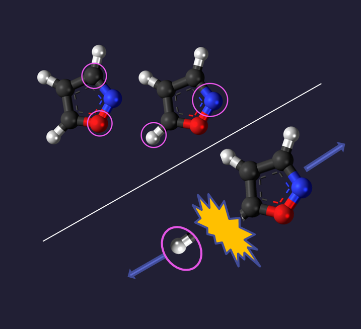
Coulomb Explosion Imaging (CEI) allows us to gain insight into the structure and dynamics of molecules. The idea behind this method is to “explode” the molecule by multiply ionizing it with a strong laser pulse and to deduce the molecular structure from the direction and kinetic energy of the molecular fragment ions that are created in this explosion (see Fig. 1). A useful way of visualizing Coulomb explosion data is the Newton Plot, which plots the momenta of fragment ions of the molecule and, ideally, creates an almost ball-and-stick representation of it. This works very well for diatomic and triatomic molecules. However, for bigger molecules like Isoxazole (C₃H₃NO), we typically only detect half of the ions at a time. While we can still make Newton Plots, we can’t use momentum conservation to refine the image since we are missing many of the fragments. My project has been to refine these images using ‘random coincidence subtraction’ instead, allowing us to determine which structures in the plots are real effects.

Fig 1. Coulomb explosion for a 3-fold ionization of a 3-body molecule

 

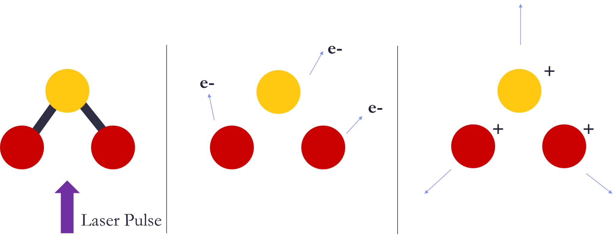
Firstly, Coulomb Explosion Imaging (CEI) uses a femtosecond laser pulse to ionize a sample. It removes an electron from each atom and causes them to all be positively charged and repel from each other coulombically. This entire process takes place in our COLd Target Recoil-Ion Momentum Spectroscopy (COLTRIMS) system. When the atoms are all charged, they are dragged by the electric field in the chamber into the detector where we measure when and where they landed.

Fig 2. Coincidence Plot for SO₂ in the S+ O+ O+ Channel, TOF 1 V. TOF 2 + TOF 3. TOF 1 means the Time of Flight for the first ion to hit the detector.

 

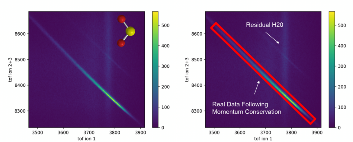
The time at which they land is related to the ions mass, charge, and momentum; and the correlation between the time of flight of several ions is also restricted by momentum conservation. On the x-axis of Fig. 2 is the time it took for the first ion to hit the detector (in nanoseconds). The y-axis is the sum of the times of the other two ions in this 3-body molecule. If the first ion landed sooner, it must have broken off towards the detector, and from momentum conservation, we know the other two must have broken away from the detector and landed later. The reverse is also true, which means we expect to see a (relatively) straight inverse relation, which is what you see with the bright line. Thus, we can remove any data that doesn’t fall near this line since it's not our molecule. Only keeping data inside the line is necessary for removing background events.

Fig 3. Coincidence Plot for Isoxazole (C₃H₃NO) in the H+ C+ N+ O+ Channel. TOF 1 Vs. TOF 2+3+4

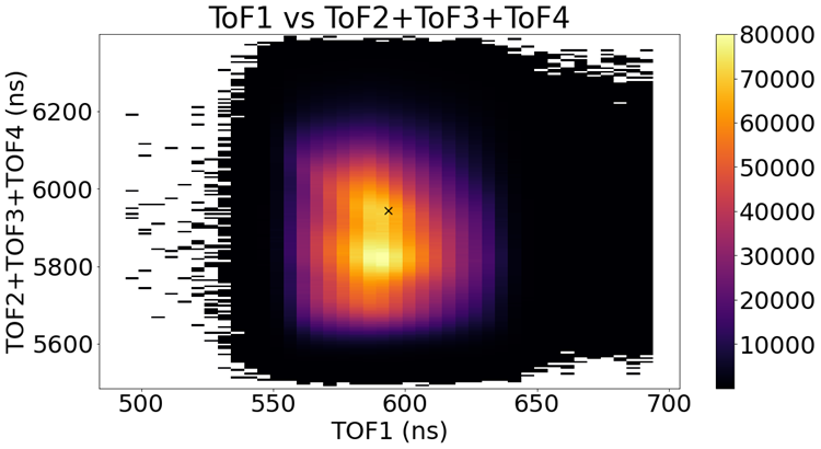
For Isoxazole, however, we only capture about half of the ions in any laser shot. This is called an ‘incomplete channel’. The graph in Fig. 3 shows the incomplete channel where each event detected what is likely an H+, C+, N+, and O+. If we don’t have the information from all of the ions, then we won’t see a bright line from momentum conservation and we can’t make any cuts from this graph to remove background data.

Fig 4. Newton Plots for SO₂ (left) and Isoxazole C₃H₃NO (right). The Isoxazole momenta are plotted from the frame of reference of the Oxygen, with Nitrogen defining the plane, and Hydrogens not plotted (thus, the dots on the right are carbons).

 

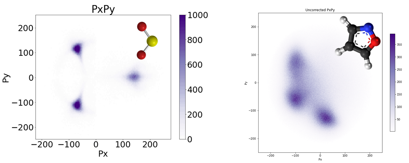
Because we know where (X and Y position) and when (Time) the ions landed on the detector, we can deduce the momentum they gained when they repelled each other.

In Fig. 4 the Newton Plot on the left is where we could subtract using momentum conservation, and the right is Isoxazole where no such cuts are made. As you can see, the Isoxazole image is ‘fuzzier’ because we couldn’t cut out data using momentum conservation.

Fig 5. Newton Plot Isoxazole C₃H₃NO with areas of interest circled.

This investigation aimed to answer why the regions circled in Fig. 5 contain a non-negligible number of carbon points. We expect three sharp spots for the carbons, yet this image indicates they could reside outside those peaks. Are these from the ‘fuzziness’ of the image or are they real effects?

Fig 6. Example of how you could collect an H+, C+, N+, and O+ from two separate molecules (top left) and how a scenario where a sample of Isoxazole being 1-7-fold ionized could produce an ion that can be detected (bottom right).

 

To combat this, we first identify the kind of ‘bad data’ we get. We want to collect an H+, C+, N+, and an O+ from one 8-fold ionized Isoxazole. ‘Bad Data’ is when at least one of the ions we collected is from a different source. This could be a second molecule that was ionized (anything from one to all of the atoms ionizing) or from residual gasses in the chamber. If T represents when a datapoint is good (True), and F is when it’s incorrect (False), all of the combinations of ways an event could be invalid are: TTTF, TTFF, TFTF, … FFFF, where TTTF represents the first three ions being correct but the fourth is wrong.

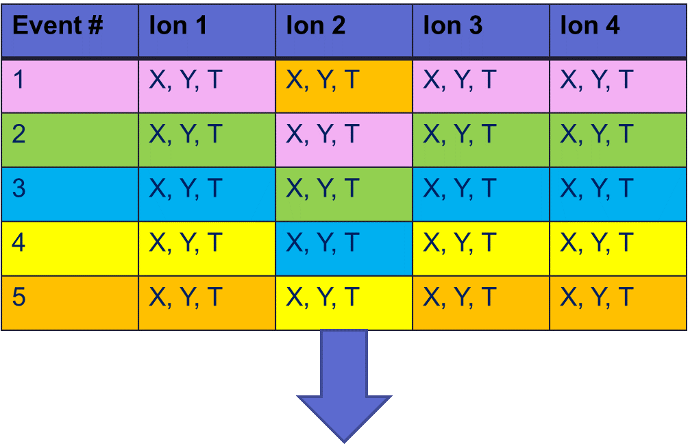Fig 7. Chart with an event number that corresponds to an individual laser pulse and the ions detected from that Coulomb explosion. Ion 2 is shifted down (out of coincidence).

 

We can model what this would look like if we ‘shift’ one ion out of coincidence (to another event). Our experiments measure ions in ‘coincidence’, meaning we know which ions came from which event. No event is related to the other, so we are replacing that ion with a random/unrelated ion in that column. There’s some probability we replaced it with a residual gas point and some probability we replaced it with a second ionization event. We do this for all the ways we could have incorrect data and finalize our model.

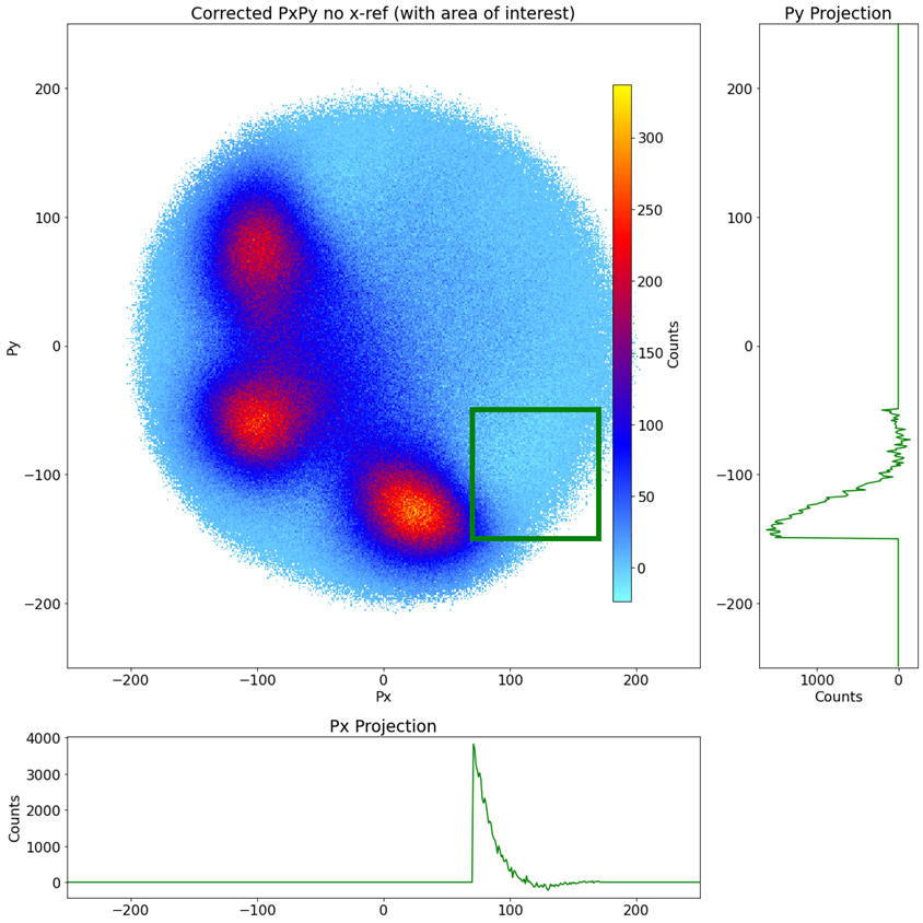Fig 8. Corrected Newton Plot for Isoxazole with Px and Py projections of the counts on the right and bottom, respectively.

Once you subtract the model from the real data, there is bound to be some pixels where the model overestimates the randoms and gives a negative-count pixel as your result. We make an approximation here and say that’s okay, so long as the overall area of the region integrates to ~ 0. To do this, we linearly scale the model down. For this specific case, 0.0303 was sufficient to fulfill this condition. Even though there are negative spots in this image, the projections on the sides show that the integrated average hovers around 0.

Fig 9. Uncorrected Newton Plot for Isoxazole Channel H+ C+ N+ O+ (left), the finalized model of the ‘bad’ data called “Boolean Model” (center), and the Corrected Newton Plot (right)

 

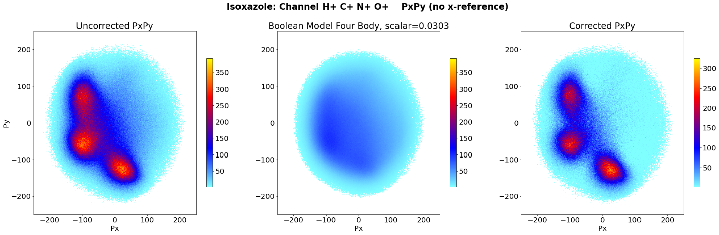
Above are our results for this summer’s project! It sharpened the image, and the model is neither isotropic nor a scaled-down version of the uncorrected plot.

Fig 10. Uncorrected Newton Plot for Isoxazole Channel H+ C+ N+ O+ (left) and the Corrected Newton Plot (right) with areas of interest noted.

 

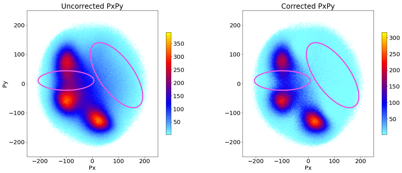
Looking at the features we hoped to explain, the carbons outside the peaks were more from background effects than real effects. The difference between the peaks and the troughs areas between them are visually and numerically larger in the corrected plot. This model extends further into plots about the kinetic energy released from the interaction, the total momenta of the fragments, and more.

Acknowledgments

I am deeply grateful for this experience, especially for the privilege to have been mentored by Daniel Rolles. Thank you to Zane Phelps, Saduni Kudagama, Tu Nguyen, Huynh Van Sa Lam, and Keyu Chen for answering any questions I had no matter how odd. And a very special thank you to Kim Coy and Loren Greenman for organizing this experience and to Kansas State University and the National Science Foundation for funding this program.

This material is based upon work supported by the National Science Foundation under Grant No. #2244539. Any opinions, findings, and conclusions or recommendations expressed in this material are those of the author(s) and do not necessarily reflect the views of the National Science Foundation.

Final Presentation