Research Project

Research Project:

Calibrating the uncertainty on the timing difference between wires and calculating the angular resolution of track-like objects

Goal:

My goal was to create detector independent filters to be added to the LArSoft framework. These filters calibrate the uncertainty on the timing difference between the wires in a LArTPC detector and then uses that measurement to calculate the angular resolution of track-like objects.

I created a way to determine the local spatial resolution of the detector from the (simulated) data. This resolution then determines how well the momentum vectores in every interaction within the detector can be measured.

Jargon:

LArSoft (Liquid Argon Software) is the software created by Fermilab for their liquid argon experiments.

To read more about this, please go here.

LArTPC (Liquid Argon Time Projection Chambers) are used for researching long base-line neutrino oscillation physics.

A TPC is a type of particle detector.

To read more about this, please go here.

Why Argon?

Argon is a noble gas (chemically inert and chemically tightly bound.)

It is also dense and clear, and argon also scintillates.

And, most importantly since a large quantity of Argon is needed (175 L for ArgoNeuT and much great quantity for MicroBooNE), Argon is cheap.

What are Neutrinos?

Neutrinos are small, sub-atomic particles that have neutral charge and interact via the weak force.

Neutrinos come in three types, known as flavors: electron neutrinos, muon neutrinos, and tau neutrinos. There is a large abundance of neutrinos. They come from the sun, from cosmic rays, from nuclear reactors, and from accelerators (to name a few.)

Interestingly, Neutrinos can change flavor. This is seen in Neutrino Oscillation Physics and Neutrino Mixing. The three different neutrino flavors can be thought of as three different mass states (eigenstates.) When an accelerator creates a beam of neutrinos, the neutrinos created can change flavor. A neutrino that changes flavor went through a mass shift; such a shift is caused by the interaction of the masses, not from the weak force. The mixing of mass states is the mixing of flavors. A neutrino that travels some distance and is created by an accelerator (neutrino beam) can be part electron neutrino, part muon neutrino, and part tau neutrino.

I encourage anyone who is interested in this to do some reading on the topic.

ArgoNeuT and MicroBooNE:

ArgoNeuT and MicroBooNE are two of Fermilab's LArTPCs.

For my project, I worked with ArgoNeuT because the software runs faster (smaller detector.) Because I have kept my code detector independent, my filters should work with any LArTPC.

For my project, I needed to learn about the wire places inside the TPC. ArgoNeuT has two wire planes (induction and collection plane) vs. MicroBooNE's three (two induction and one collection planes) that are at 60 degrees to each other.

To learn more about ArgoNeuT, please go here.

My Project:

As mentioned above, I created my project so that it is detector independent. Because both parts of my project rely on how many planes a detector has (ArgoNeuT 2, MicroBooNE 3), both of my filters extract the number of planes and then formats the rest of the code to accept that number.

The first part of my research project was to create a filter that calibrates the uncertainty on the timing difference between wires in the TPC. The timing differences between the wires should be around zero, meaning the time between wires 1 and 2 should be almost equal to the time between wires 2 and 3. My results proved this to be true.

To do this, I first had to be able to pick out level tracks in the Argon. A level track is any track that has a starting point and ending point that is the same distance away from the wire planes. What is a track? For my project, I worked with high energy muons. When high energy particles travel very fast through a medium (in this case muons traveling through Argon), they leave a track of ionized particles. My tracks, therefore, were the particles ionized by a fast moving muon.

To first filter out level tracks from non-level tracks, I had to calculate the angle a track makes. I then set a threshold value: anything below my threshold is considered a "good" track (threshold in most cases is 5 Degrees, but it can vary.)

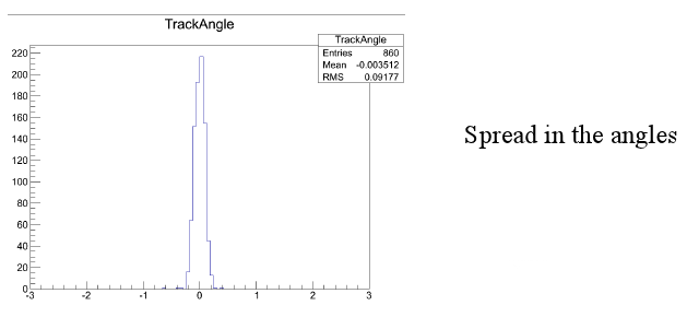
The above histogram shows the spread in the angles of the "good" tracks (number per bins vs radians.)

Once a track is determined to be level, I began extracting the information from the track; ie, what composes the tracks. If you remember from above, a track is the ionized particles in the TPC from a high energy muon. Meaning, a track is composed of all the hits from these particles on the wire planes. And what is a hit? A hit is a wire number and a time (essentially where and when.)

To recap, a track is a path of ionized particles. These ionized particles hit certain wires at specific times in the wire plane.

From each track I made a sorted vector (c++) of wire numbers and peak hit times. Each vector was then filtered based on unique consecutive pairs and unique consecutive triples (if wires were skipped or wires had more than one hit, that wire number and time were discarded.)

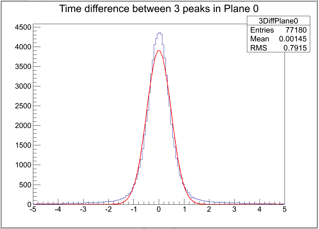
Above you see the histogram of the time differences between unique consecutive triple wires with a Gaussian fit to the curve. As expected, the mean is very close to zero.

This, though, represents ALL the timing differences for ALL the hits along a track. To analize this, I needed to look at all the timing differences for specific time ranges. Because of the way ArgoNeuT is designed, the detector takes 2048 readings which I then divided into eight separate regions.

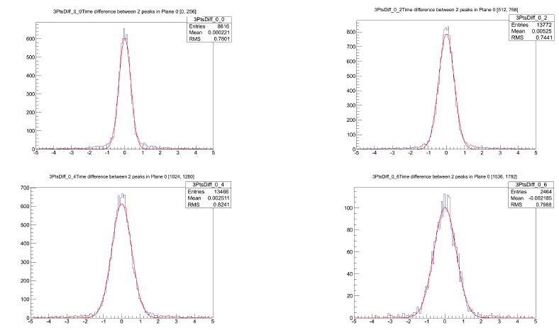
REGION 1, 3, 5, 7

The four histograms above represent the timing differences between unique consecutive triple wires in regions 1, 3, 5, and 7 with the time range (0-2048) listed.

The important thing to notice here is the spread in the curves as the track goes along. Region 7 has a much broader curve than Region 1 (a mean of about .8 vs a mean of about .0002), which is expected because of the drift physics (mainly diffusion.)

From these eight histograms, I calculated the error on each one to make the following plots:

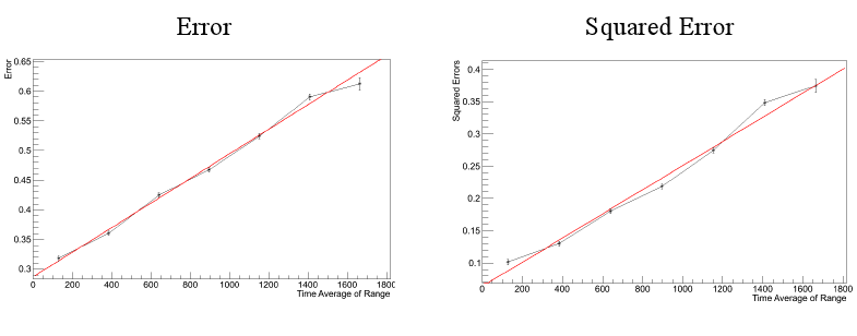
These two graphs are the error and the squared error from the eight histograms plotted against its respective time range. The error increases linearly with time, which is also expected. The total error is the diffusion error (slope of graph) plus the resolution error (intercept of graph.)

These two errors were a necessary measurement for the second part of my project.

The second stage of my research project was to calculate the angular resolution between tracks. By having a calculation of what the local spatial resolution error is, I could by similar methods extract track information, take the inverse of a 2x2 matrix composed of the second partial derivatives of chi squared with respect to the time and the angle to determine the wire and angular resolution.

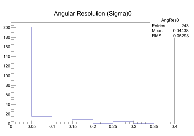
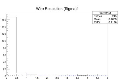
From these histograms, the angular resolution can be measured to be roughly .032 radians or 1.8 degrees, and the wire resolution to be around 1 wire.

This means, two tracks can be differentiated to within 1.8 degrees and to within 1 wire. This calculation is important because a track cannot be distinguished to anything below the uncertainty on it (in this case, within 1.8 degrees and 1 wire.)

This is very useful for Small Angle Scattering.