|
Forecasting ability of a periodic component extracted from
large-cap index time series-Comparison of the repetition function method of
finding a periodicity with two other methods using test data. M. J. O’Shea, Jour. Forecasting
To
illustrate the repetition function method and compare to the
autocorrelation function and spectral density methods we created three
price time series using the business days from Jan. 2nd 1930 –
Jan. 2nd 2015.
A1.1 Generating the test time series
Three
test time series are generated. Each time series P(t) is
made up of a constant term P0, a non-periodic term PNPr(t)
increasing at approximately 7 price units per year, a stochastic term PS(t)
of average amplitude AS = 2 price units and a periodic
term PPr(t) who’s average amplitude is different
for each of the three series. Figure A1(a) shows a section of the test
time series consisting of the sum of the first three terms only.
The
periodic term, PPr(t) is chosen to be a narrow
rectangular pulse of width 10 days. To keep the test data as general as
possible the amplitude of the pulse is varied at random and allowed to be
negative but with an average (positive) amplitude APr as
illustrated in Figure A1(b). The midpoint of the pulse is placed as close
as possible to the arbitrarily selected 8th day of November of
each year. Thus it is not precisely periodic since the length of a year
varies by a few days from year to year. Its periodicity averages to 252
business days. The average amplitude, APr, of the
periodic term (chosen to be much smaller than the change in the
non-periodic term over one year) is 2.0, 1.0 or 0.4 price units for the
three series so that the ratio APr/AS
for the three test series is 1.0, 0.5 and 0.2.
A1.2. The autocorrelation method
The
autocorrelation method can be used to infer if a periodicity is present in
a time series. It is convenient to differentiate P(t) to
remove most of the effect of the non-periodic background. Since the
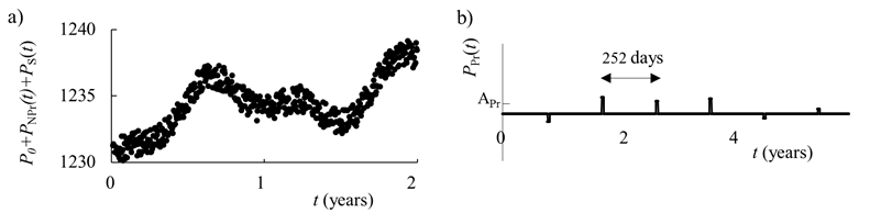
Figure
A1. The generated test data. a) A two-year section of the generated
85-year test time series consisting of a constant P0, a
non-periodic term PNPr(t), and a stochastic term PS(t)
of amplitude AS of 2 units. b) A 6-year section of the approximately
periodic part of the time series, PPr(t), of average
period 252 business days (1 year) with average amplitude APr.
The test data of a) are combined with the test data of b) (with three
different amplitudes APr = 2.0, 1.0 or 0.4 price units) to
make the three test data time series.
data is noisy, it must be
smoothed prior to differentiating. Several different combinations of
smoothing and differentiating were tried and it was found that a
straightforward five-point smooth before differentiating worked best. j(t) is then
calculated from the change in adjusted closing price per day, dP(t)/dt
:
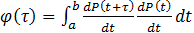 (A1) (A1)
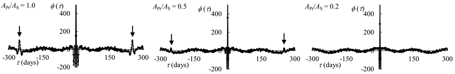
Figure
A2. The autocorrelation function for the three sets of test data. Arrows
indicate a time of ± 252 days. No autocorrelation peak is present for
the case APr/AS = 0.2.
This
calculated correlation function is shown in Figure A2 for each of the three-time
series. A large sharp self-correlation peak is centered att = 0 and decays away to a background value of
approximately  for t ≠
0. An autocorrelation peak is present at t = ± 252 days as
indicated by the arrows for the case of APr/AS
= 1.0. When the amplitude of the periodic term is reduced (APr/AS
= 0.5) the correlation peaks are just vanishing into the background noise
in f(t) and for
the smallest amplitude (APr/AS = 0.2)
no correlation peak is visible. for t ≠
0. An autocorrelation peak is present at t = ± 252 days as
indicated by the arrows for the case of APr/AS
= 1.0. When the amplitude of the periodic term is reduced (APr/AS
= 0.5) the correlation peaks are just vanishing into the background noise
in f(t) and for
the smallest amplitude (APr/AS = 0.2)
no correlation peak is visible.
A1.3. Fourier analysis and the spectral density
Any time-series  that is of the form of a periodic function can be
represented by a sum of components in the form of sines and cosines or by a
sine function with a phase shift that is of the form of a periodic function can be
represented by a sum of components in the form of sines and cosines or by a
sine function with a phase shift  : :
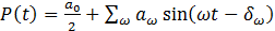 , ,
provided
that is reasonably well behaved.
If the mean value of the time series is zero then a0 =
0. The sum over frequency w is usually
the sum over a fundamental frequency w0 and harmonics 2w0 , 3w0 etc. In our test data the fundamental frequency
of the periodic component corresponds to a period T0 of
252 business days and the phase is also known. Using w = 2p/T and with the change of notation aw ® aT,
the coefficient aT is given by:
 . .
This
is the spectral density and yields the amplitudes of periodic terms that
contribute to the time series. In practice the integral is done over many
periods, T. The price time series was scaled so that if the only term present in
the time series was 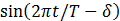 , then , then  would be 1. We performed this analysis on our
test data of the previous section and would be 1. We performed this analysis on our
test data of the previous section and  vs T for these time series are shown in
Figure A3. In these plots we varied the period T about the known
value of 252 days and a small peak connected vs T for these time series are shown in
Figure A3. In these plots we varied the period T about the known
value of 252 days and a small peak connected
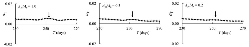
Figure
A3. The coefficient versus period T for our test data. Arrows
indicate the expected position of a component (peak) signifying a
periodicity of 252 days. No peak is present for the case APr/AS
= 0.2.
with
a periodicity of 252 days is found for our test time series with the
largest periodic contribution
(Apr/AS
= 1.0). As the periodic contribution to the time series decreases this
peak gradually vanishes. The reasons these peaks are small is a combination
of:
·
the periodic
term only contributes a small amount (approximately 4%) to the magnitude
of the time series, most of the time series magnitude comes from large
stochastic and other non-periodic contributions.
·
the amplitude
of the periodic term varies from year to year.
·
the exact
period varies slightly from year to year since different years have
different numbers of business days.
Several
modifications of this analysis were tried including various types of data
smoothing and none proved successful in identifying a periodic component
for Apr/AS = 0.2.
In
addition to the above problems a second harmonic contribution (at T
of 126 days) was not detectable. For the spectral analysis method to
reveal the shape of the periodic term, we would need to detect the peak
associated with the fundamental period and several of its harmonics to
reconstruct the periodic contribution to this time series and this does not
prove to be possible.
A1.4. The repetition function method
This section should be read along with Section 2
of our paper. To calculate the repetition function we take the tk to
be the first business day of each year and it is convenient to measure t
and tk from
an origin of Jan. 2nd 2015 so that t1 = 0,
t2 =
252, t3 =
504, t4 =
754 days etc. Construction of the repetition function via equation (5)
significantly reduces any stochastic contribution from the time series. It
also averages over any non-periodic variation in the time series to produce
a linear term. The repetition function for each of the three-time series
is shown in the top three plots of Figure A4. The percent change in  , i.e. , i.e. 
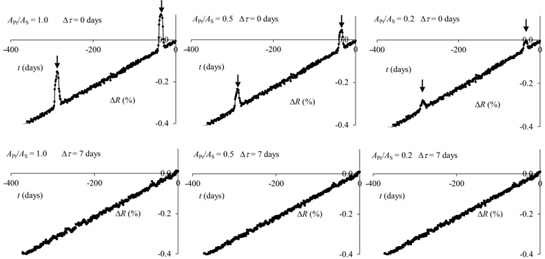
Figure
A4. The repetition function for the three sets of test data. The tk of
equation (5) are set to the first business day of each year. Repetition
functions are shown for test data with APr/AS
= 1.0, 0.5 1oise (S/N) ratio of of the
background. or of y is more apparent in the repetition function sinc ethe
sting that the presencand 0.2, and Dt is set
equal to zero days or seven days as indicated. The arrows are spaced by
252 days and the presence of the indicated peaks (upper plots) show that a
periodicity is detectable for all three test data series. When Dt is not zero (lower plots) the periodicities
vanish for all three test series as expected.
 , is plotted. The periodic signal is easily found
for each of the time series and indicates the repetition function is more
sensitive than the autocorrelation function or spectral density method in
finding periodicities and reconstructing this component. The overall
linear increase of the background in the repetition function results from
the long-term uptrend in our test data. The position of the periodic
signal in the repetition function is found to be Nov. 8th as
expected. , is plotted. The periodic signal is easily found
for each of the time series and indicates the repetition function is more
sensitive than the autocorrelation function or spectral density method in
finding periodicities and reconstructing this component. The overall
linear increase of the background in the repetition function results from
the long-term uptrend in our test data. The position of the periodic
signal in the repetition function is found to be Nov. 8th as
expected.
If the period is not chosen to be a periodicity
that is present in the price function, P(t), then the
repetition function should yield only linear and stochastic terms along
with a constant background. Thus when a periodicity is found, it should be
possible to change that periodicity by a small amount Dt , see equation (5), so that the repetition
function no longer has a periodic component. This serves as a check on
this method. The repetition function with Dt set to 7
days is shown in the lower plots of Figure A4 for our three sets of test
data. A periodic component is no longer present as expected.
While
the first time period in the repetition function, i.e. the first 252 days,
has complete overlap allowing signals to add up, this will not happen for
time periods further from the origin since the term PPr(t)
is not exactly periodic. Thus sharp signals close to the origin will be
superimposed by the
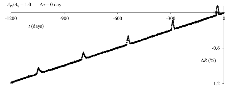
Figure
A5. The repetition function over an extended time range. The tk of
equation (5) are set equal to the first business day of each year. The
amplitude of the peak is gradually reduced for peaks further from the
origin due to the fact that the test data is not exactly periodic in time.
repetition function and
add coherently while sharp signals further from the origin may not add
coherently. This effect can be seen in the repetition function of Figure
A5 for APr/AS = 1.0 plotted over an
extended time range. The maxima further from t = 0 are reduced in
amplitude with a reduction of about 10 percent per maxima.
In
conclusion the repetition function is more likely than the autocorrelation
method or the spectral density method to reveal a periodicity provided one
knows the particular periodicity to search for. This is due to the
reduction in the stochastic contribution and the averaging of non-periodic
variations over many time periods as the repetition function is constructed
via the summation in equation (5).
|