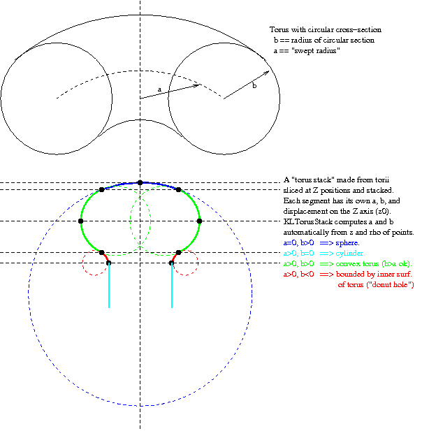
n of segments in the stack.. The array parameters are named z_edge, rho_edge, and z_o. The first two arrays are n+1 long, and define the points at which the segments join. The z_o array is n elements, and defines the Z position of the center of curvature of each segment. The following diagram (taken from the Hamamatsu PMT manual, with annotations added by hand in green), should help make this more clear:
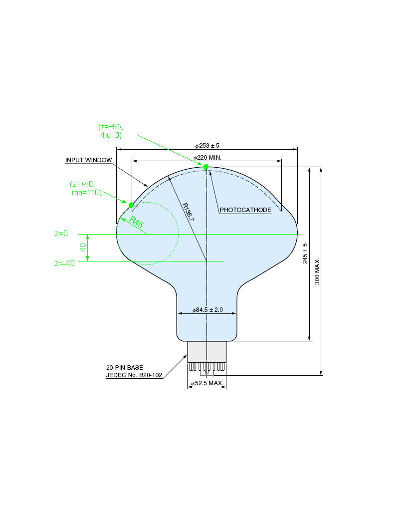
z_o for the first segment, z_o[0], should be -40. The first segment begins at about z=+95 mm, rho=0 mm. The first segment ends, and the second segment begins, at z=+40, rho=110. The center of curvature of the second segment is right on the equator, so z_o[1]=0. The second segment ends at z=0, rho=253/2=126.5. So the values for the first two segments are (approximately)
   z_edge[]   = { 95,     40,      0.0 ... }
   rho_edge[] = {  0,    110,    126.5 ... }
   z_o[]      = {    -40,      0,      ... }
TorusStack is able to compute values of "a" and "b" for each segment from z_edge, rho_edge, and z_o. Note that in the example above, it would actually end up calculating a value of a=135 mm for the first segment (not 136.7) because we specified the top of the first segment to be at z=+95 and the center of curvature to be at z_0=-40.
If there is some inconsistency in the input parameters, TorusStack does the best it can to resolve it and prints out a warning message.
TTree's, named event_tree and run_tree. All of the basic ROOT functions for inspecting the structure of TTree's, such as Print(), Show(), and Scan() work as usual. See the ROOT documentation for more. Due to the use of C-style structures and some oddities that haven't been fully understood yet, the TTree::GetBranch() function may not always be as useful as it is supposed to be. TTree::GetLeaf() seems to work, at least in cases where the leaf name is unambiguous. TTree::Draw() also works, and seems to always find the leaf you want, making use of the branch names as you would expect. Furthermore, TTree::Draw() is more useful than you might think due to the TTree::GetVar*() functions.Here's an example ROOT session demonstrating some of these functions:
root [0] TFile f("my_test_run.root")
root [1] event_tree->Draw("hit_time","hit_count")
<TCanvas::MakeDefCanvas>: created default TCanvas with name c1
(Int_t)249217
root [2] event_tree->GetV1()
(Double_t*)0xb781c008
root [3] event_tree->GetV1()[0]
(Double_t)2.26637983888417480e+01
root [4] event_tree->GetV1()[1]
(Double_t)2.46895360891042479e+01
root [5] event_tree->GetV1()[2]
(Double_t)1.44446145343176759e+01
root [6] event_tree->Scan("hit_time:hit_count")

    Row   * Instance *  hit_time * hit_count *

        0 *        0 * 22.663798 *         1 *
        0 *        1 * 24.689536 *         1 *
        0 *        2 * 14.444614 *         1 *
        0 *        3 * 25.442434 *         1 *
        0 *        4 * 7.7838687 *         1 *
        0 *        5 * 8.6318399 *         1 *
        0 *        6 * 9.9425388 *         1 *
        0 *        7 * 10.089205 *         1 *
        0 *        8 * 10.489053 *         1 *
        0 *        9 * 13.112237 *         1 *
        0 *       10 * 15.506406 *         1 *
        0 *       11 * 17.058913 *         1 *
        0 *       12 * 18.827770 *         1 *
        0 *       13 * 19.363745 *         1 *
        0 *       14 * 22.467745 *         1 *
        0 *       15 * 23.598506 *         1 *
        0 *       16 * 24.931971 *         1 *
        0 *       17 *   33.0238 *         1 *
        0 *       18 * 35.734850 *         1 *
        0 *       19 * 19.936568 *         1 *
        0 *       20 * 24.164396 *         1 *
        0 *       21 * 24.610297 *         1 *
        0 *       22 * 32.300285 *         1 *
        0 *       23 * 8.8683131 *         1 *
        0 *       24 * 8.9568964 *         1 *
Type <CR> to continue or q to quit ==> q

(Int_t)25
root [7] event_tree->Show(0)
======> EVENT:0
 fStartRealTime  = 1.10866e+09
 fStopRealTime   = 1.10866e+09
 fStartCpuTime   = 0.59
 fStopCpuTime    = 5.2
 fTotalCpuTime   = 4.61
 fTotalRealTime  = 4.64721
 fCounter        = 1
 fUniqueID       = 0
 fBits           = 50331648
 eventID         = 0
 runID           = 0
 UT              = 3.36973e+08
 delta_UT        = 3.36973e+08
 eventType       = 3
 n_particles     = 1
 t0              = 0
 x0              = -1350
 y0              = -60
 z0              = 270
 pdg_code        = 2212
 px              = 0
 py              = -162.689
 pz              = 0
 polx            = 0
 poly            = 0
 polz            = 0
 ke              = 14
 vketot          = 14
 vcentroid_x     = -1350
 vcentroid_y     = -60
 vcentroid_z     = 270
 n_photon_hits   = 1937
 hit_time        = 22.6638,
                  24.6895, 14.4446, 25.4424, 7.78387, 8.63184,
                  9.94254, 10.0892, 10.4891, 13.1122, 15.5064,
                  17.0589, 18.8278, 19.3637, 22.4677, 23.5985,
                  24.932, 33.0238, 35.7349, 19.9366
 hit_pmt         = 175,
                  175, 523, 523, 311, 311, 311, 311, 311, 311, 311,
                  311, 311, 311, 311, 311, 311, 311, 311, 296
 hit_count       = 1,
                  1, 1, 1, 1, 1, 1, 1, 1, 1, 1,
                  1, 1, 1, 1, 1, 1, 1, 1, 1
 n_pmt_hits      = 1940
 n_hit_pmts      = 467
 totScintEdep    = 14
 totScintEdepQuenched = 7.52104
 scint_centroid_x = -1349.99
 scint_centroid_y = -61.492
 scint_centroid_z = 270.027
root [8] TLeaf*l_time= event_tree->GetLeaf("hit_time")
root [9] l_time->GetNdata()
(const Int_t)1937
root [10] l_time->GetValue(0)
(const Double_t)2.26637983888417480e+01
root [11] l_time->GetValue(1)
(const Double_t)2.46895360891042479e+01
root [12] l_time->GetValuePointer()
(const void*)0xa371050
event_tree data is the most interesting of the two trees. It contains the following information:
| TStopwatch | event_timer | Elapsed CPU and real time |
| Double_t | fStartRealTime | event_timer variables |
| Double_t | fStopRealTime | |
| Double_t | fStartCpuTime | |
| Double_t | fStopCpuTime | |
| Double_t | fTotalCpuTime | |
| Double_t | fTotalRealTime | |
| Int_t | fCounter | |
| Int_t | fUniqueID | |
| Int_t | fBits | |
| Int_t | eventID | event number |
| Int_t | runID | run number |
| Float_t | UT | Simulation "Univeral Time" in ns |
| Float_t | delta_UT | time since last event, in ns |
| Int_t | n_particles | number of particles in vertex |
| Float_t | t0[n_particles] | info on primary vertex particles |
| Float_t | x0[n_particles] | |
| Float_t | y0[n_particles] | |
| Float_t | z0[n_particles] | |
| Int_t | pdg_code[n_particles] | |
| Float_t | px[n_particles] | |
| Float_t | py[n_particles] | |
| Float_t | pz[n_particles] | |
| Float_t | polx[n_particles] | |
| Float_t | poly[n_particles] | |
| Float_t | polz[n_particles] | |
| Float_t | ke[n_particles] | |
| Double_t | vketot | Total kinetic energy in primary vertex |
| Float_t | vcentroid_x | Energy-weighted "centroid" of primary vertex |
| Float_t | vcentroid_y | |
| Float_t | vcentroid_z | |
| Int_t | n_photon_hits | Number of photon hits (photoelectrons detected) |
| Double_t | hit_time[n_photon_hits] | Time of hit |
| Short_t | hit_pmt[n_photon_hits] | Index of PMT hit |
| Int_t | hit_count[n_photon_hits] | integer hit "weight" -- hit should be counted this many times |
| Int_t | inner.n_pmt_hits | number of photon hits in inner detector |
| Int_t | inner.n_hit_pmts | number of inner pmts with 1 or more hits |
| Int_t | outer.n_pmt_hits | number of photon hits in outer detector (your geometry may not have this) |
| Int_t | outer.n_hit_pmts | number of outer pmts with 1 or more hits |
| Float_t | totScintEdep | Total energy deposit in scintillator |
| Float_t | totScintEdepQuenched | Birks-law-quenched energy deposit sum (see question below) |
| Float_t | scint_centroid_x | Quenched-energy-weighted centroid of scintillator energy deposit position |
| Float_t | scint_centroid_y | |
| Float_t | scint_centroid_z |
dS = k dE / (1 + kB dE/dx)
The quenched energy in GLG4sim -- let's call it "E_Q" -- is defined by
dE_Q = dE / (1 + kB dE/dx)
So to answer your question, "totScintEdep" is the total energy deposited in the scintillator, i.e. the integrated dE, and "totScintEdepQuenched" is the quenched energy deposit, i.e. the integrated dE_Q.
The total amount of light emitted in the scintillator is proportional to totScintEdepQuenched, and the number of photon hits obtained from an energy deposit at a given position is proportional to the amount of scintillator light, so in that sense the number of photon hits "corresponds" to totScintEdepQuenched. But of course the exact number of photon hits you get for a given quenched energy deposit depends on position of the energy deposit in the detector, attenuation lengths, orientation of the PMTs, etc.
 1.3.9.1