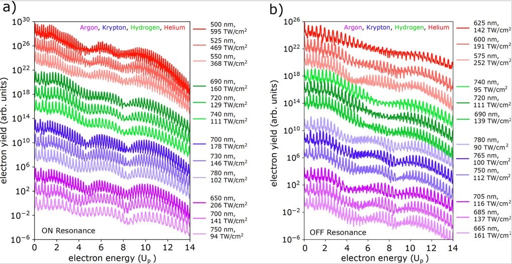
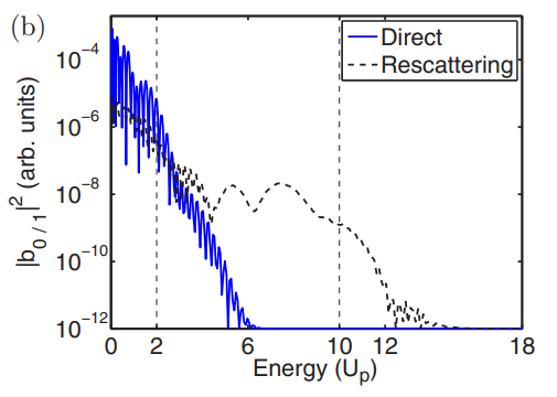
When atoms are exposed to an intense laser field, electrons are removed from the atoms by direct ionization or by indirect rescattering processes. Elastically rescattering electrons are created by a three-step process. The first step is the tunnel ionization when the pulse first hits the atom, in which an electron is ejected from the atom. Then, due to the oscillating electric field, it is accelerate back towards the atom. In the third step the electron passing through the atomic ion is further scattered away. One can get the photoelectron energy spectra for the rescattered electrons, and for certain half-integer N in the resonance condition, there will be an enhancement in electron yield for specific ranges of energies. This enhancement, additionally, is universal across different laser parameters and also different target elements (if they still yield half-integer solutions to the resonance equation, see figure one.). There is currently a large effort to understand these enhancements: why do these specific energy ranges yield such enhancements, and why do they occur. For integer N, however, the enhancement nearly completely disappears. My goal for the summer was to perform simulations to model the direct electron scattering and electron rescattering under an ultrashort intense laser pulse, and to obtain the photoelectron energy spectra graph.

Fig. 1: Energy distribution of rescattered electrons under various ultrafast laser pulses.

For our target element, we chose Argon for its low ionization energy. Our first task was to construct the ground state electronic wave function. To do this, we used the Renormalized Numerov Method with a soft-core Coulomb potential -(z² + a²)^1/2. The Numerov method will take a given ionization energy and determine which possible a value gives a solution to the time-independent Schrödinger equation. Each atom has its own unique a value for the soft-core Coulomb potential, and once it is determined, we have an accurate approximation of the potential energy from a given atom. In this case, we have the potential for argon and helium. Using these potentials, you then can get the wave functions for electrons in the first few excited states, as well as their respective energy levels.

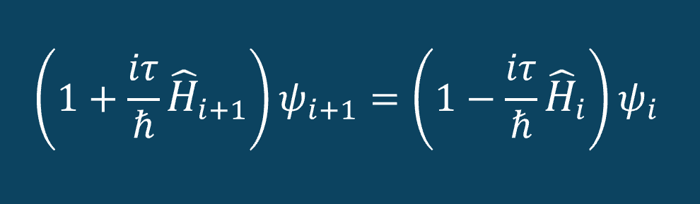
Once we obtained the ground state wave function for an electron in helium, we then used the Crank-Nicolson algorithm to propagate the wave function over time. (See figure two) It takes a wavefunction at a given time step and outputs the wave function for the next time step. To do this, we construct the Hamiltonian matrix as input into the driver equation for the Crank-Nicolson algorithm. We utilized the 5-point stencil method for the construction of the Hamiltonian in order to approximate the second derivative of the wave function at each time. Since we know the potential energy at each time step, we know the exact Hamiltonian at each time step. Then, we can propagate the wave function over any range of time that we desire.

Fig. 2: Main driver equation of the Crank-Nicolson algorithm. τ is the time step of the simulation and is the Hamiltonian matrix.

 

First, to benchmark our simulation, we modeled the ionization of an electron under atomic potential and a constant electric field. To do this, we took an initial electron in a ground state under potential energy from helium and considered an electric field of the form xE₀ . We ran the simulation from -25 to 25 fs, turning the induced electric field off when time equals 0. The electron’s wave function initially starts out in as a Gaussian shape (since it is in the ground state under the potential from one atom), and when the simulation begins, a small wave packet is generated. (See figure three)

Fig. 3: Wavefunction of ground state electron in Argon under a constant electric field that is equivalent of a laser of intensity of 100 TW/cm² laser that is turned off when time equals 0. The wavepacket that gets ejected to the left represents the probability of ionization of the electron.

 

This represents the ionized electron as it travels away from the atom. The probability of ionization of an electron is given by the area under the modulus square of the wave function in the asymptotic region. We carried out this process for several different electric field intensities and compared it to what is known as the Ammosov-Delone-Krainov (ADK) model for the ionization of electrons. (See figure four)

Fig. 4: Probability of ionization for a ground state electron in a Helium atom under a range of laser intensities.

 

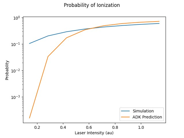
ADK theory was used to calculate the predicted probability of ionization for the same set of electric field intensities that we used in the simulation. The large gap between the ADK predicted probability values and the simulation predicted values in the low intensity regime can be explained by ADK theory’s low accuracy for low intensity regimes. In the low intensity regime, ADK theory is known to have poor accuracy when predicting ionization probabilities, but much higher accuracy in the higher energy regimes.

Once it was verified that the simulation is accurate for directly scattered electrons. We moved to calculate time-dependent electron wave function under the ultrafast laser pulse by solving the time-dependent Schrodinger equation. We modeled the laser pulses with a Gaussian envelope multiplied by a cosine term. The first part is to specify the general shape of the laser pulse, while the second part is the oscillating term. We followed the same process that we did with the static laser to obtain the wave function of the electron over time. (See figure five)

Fig. 5: Wavefunction of ground state electron in Argon under a 150 TW/cm² and 800 nm laser pulse. The wavepackets that get ejected to the left and right represent the probability of ionization of the electron.

 

An important aspect to take note of is that ejected wave packets, in the beginning of the simulation, get turned around and set back at the atom. This represents the step of the previously described electron rescattering. From the wave function in coordinate space, we can obtain the wave function in momentum space by Fourier transform. This will then give us the photoelectron energy distribution, which was the main goal of the project.

The energy spectra distribution that we currently have, however, is not at all what it is expected to look like. (See figure six)

Fig. 6: The top graph is the current energy distribution I have for rescattered electron, while the bottom graph is the expected energy distribution. Although the bottom graph has bottom directly scattered and rescattered electron energy distributions, we only have a rescattered energy distribution, so that is what we compare with.

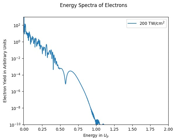
There is a sharp drop in the distribution of my simulation’s energy spectra after 0.7 Up, which is completely unexpected. This means that the production of the energy distribution needs to be reworked. So, future work on this project will entail that. Some possible fixes to the energy distribution problem could be a larger simulation box, a smaller time step, or even dropping the Crank-Nicolson algorithm for a more accurate TDSE propagation algorithm.

Citations

Blaga, Kansas State University AMO Seminar, November 2022

https://github.com/aychun/Crank-Nicolson-Method-for-Time-Dependent-Schrodinger-Equation

Noslen Suárez, Alexis Chacón, Marcelo F. Ciappina, Jens Biegert, and Maciej Lewenstein

Phys. Rev. A 92, 063421 – Published 28 December 2015

Acknowledgements

I would first like to thank Professor C.D. Lin and Isaac Yuen for their mentorship, patience, and commitment to helping me improve as a physicist throughout the course of this project as they welcomed me to their team. I am grateful to Kim Coy, J.T. Laverty, and Loren Greenman for their roles in organizing this program and assisting me with kindness, as well as Kansas State University and the National Science Foundation for funding this unforgettable experience.

 

Final Presentation