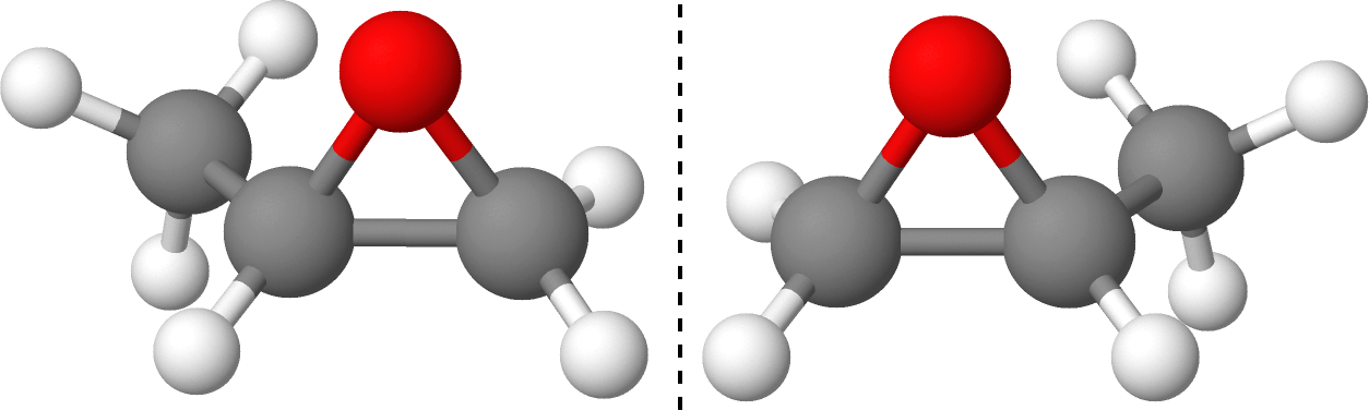
Chiral molecules (Fig. 1) are molecules with non-superimposable mirror images, called enantiomers. Many biological molecules are chiral, so the ratio of enantiomers in a solution (called enantiomeric excess) can be vital for drug synthesis. Due to breaking parity symmetry, chiral molecules will interact differently with different polarizations of light. When circularly polarized light is used, this effect is called circular dichroism. Traditionally, circular dichroism is measured through absorption based techniques, but this provides a relatively weak signal. One way to improve this effect is by ionizing the chiral sample and catching the electrons. The differential photoelectron angular distribution obtained through ionization with circularly left and right polarized light is called photoelectron circular dichroism (PECD). Our goal is to accurately model and optimize PECD signals.

Fig. 1. Propylene oxide (methyloxirane). A simple, yet widely-studied chiral molecule. The chirality of methyloxirane can be seen in the exchange of CH3 with hydrogen in the back of the molecule. This is also the molecule with which the calculations for this project are performed.

 

Our model for PECD requires three steps for calculation. First, we perform a quantum chemistry calculation with a program called Molpro, which finds the approximate molecular wave function. We use the Hartree-Fock method to find the single electron wave functions called orbitals, which are linear combinations of Gaussian functions, and the total molecular wave function, which is an antisymmetrized product (called a Slater determinant) of the orbitals. The Hartree-Fock method utilizes the variational principle, which states that the expectation value of the Hamiltonian operator is greater than or equal to the actual energy of the system, as well as approximations, such as the Born-Oppenheimer approximation, which neglects nuclear kinetic energy from the Hamiltonian and the Hartree-Fock approximation, which reduces electronic interaction to the average over all electrons, to optimize the electronic orbitals for the lowest energy. The quantum chemistry calculation gives us the bound states, both occupied and unoccupied (virtual), of electrons in the molecule. The second step to calculating PECD is the scattering calculation, which is performed with a program called ePolyScat2, 3. After ionization the electron is no longer in a bound state, which has discreet energy levels, but instead enters the continuum, in which the energy can take any value. The scattering calculation describes the ionized state of the electron. The final step describes the interaction with the laser through time-dependent perturbation theory. (TDPT) This solves for the time-dependent coefficients in the N-electron wave function (Eq. 1), which gives the momentum distribution of the ionized electron (Eq. 2). Expanding Eq. 2 into associated Legendre polynomials, we end up with the anisotropy parameters (β) which are discussed frequently in this project.

(Eq.1)

(Eq. 2)

After calculating PECD, our goal is to optimize (maximize) the signals experimentalists can obtain. Previously, we have focused on multicolor pulse-shaping techniques1, in which parameters of the driving laser field are optimized. This theoretically produces much larger PECD signals, but requires challenging experimental control over XUV laser fields. This has turned our focus to implementing the reconstruction of attosecond beating by interference of two-photon transitions (RABBITT) experimental technique4, in which the delays between experimentally attainable pulses can be controlled for optimization. The RABBITT technique involves using multiple evenly spaced XUV harmonics with a singular IR pulse, in which the delays between the pulses can be varied.

The main goal of my project this summer has been to determine the sensitivity of the results obtained from the TDPT calculation to virtual orbital energies obtained from quantum chemistry, so we can determine the robustness of the calculations. To do this, the virtual orbital energies from quantum chemistry were fit using a linear and quadratic fit (Fig. 2), and the anisotropy parameters and PECD were calculated as a function of the fit parameters. Imaginary parts were also added to the virtual orbital energies. Results from the linear, quadratic, and complex energies are shown in Figs. 3-5, respectively.

Fig. 2. The variation of fit parameters with quadratic fit. Shown in red are the virtual orbital energies directly from the quantum chemistry calculation. The blue dotted line is the line of best fit obtained with quadratic interpolation. The gray shaded region shows the energies obtained with variation of the quadratic fit parameter.

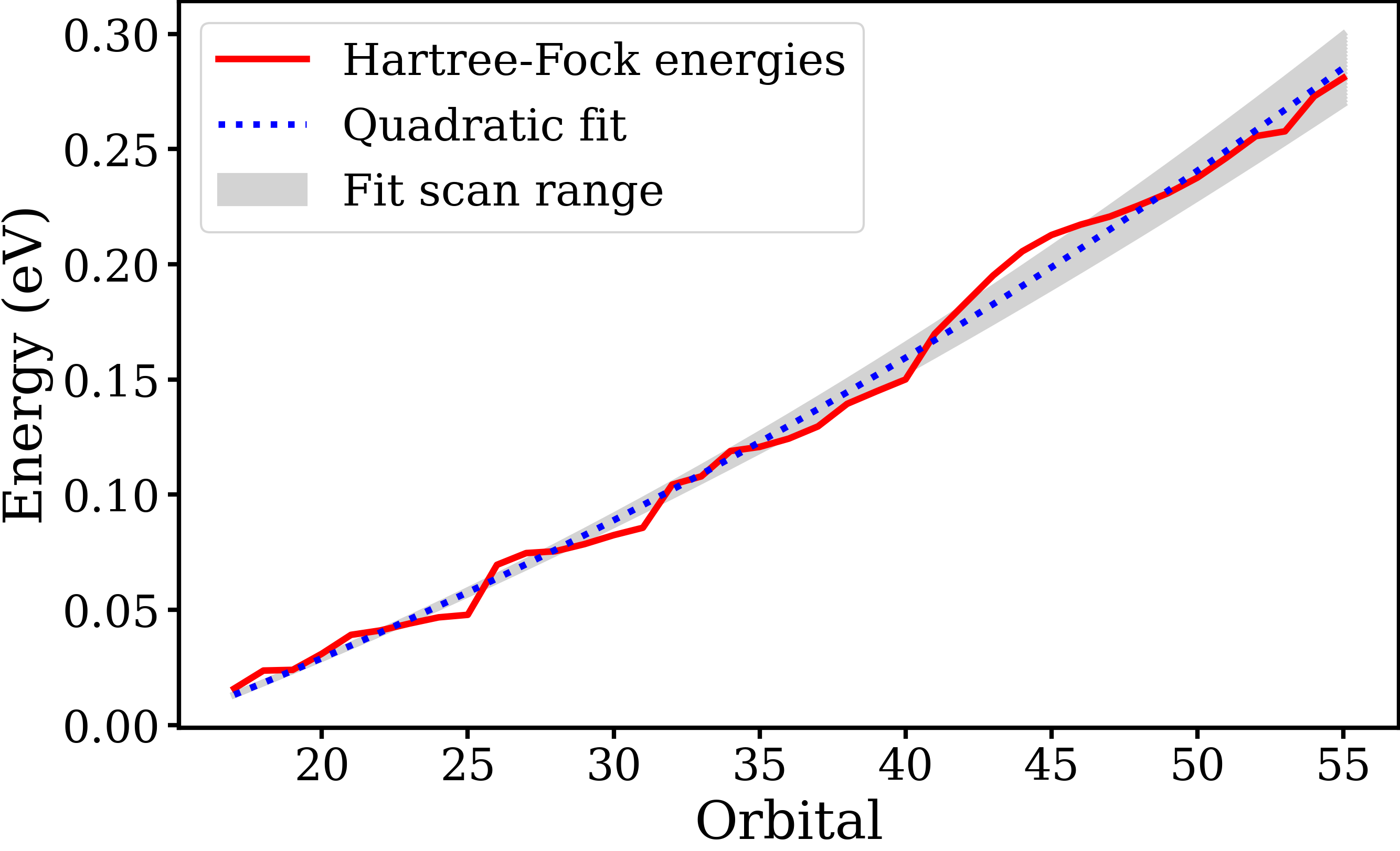
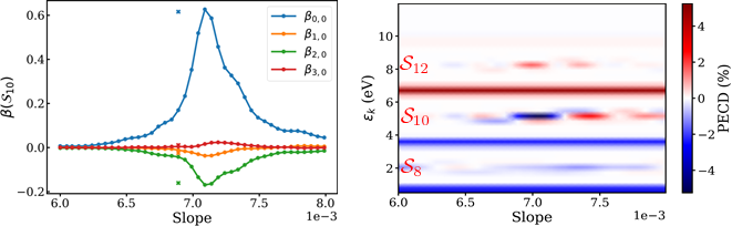
Fig. 3. Results for slope fit. The anisotropy parameters for sideband 10 (left) can be compared with the PECD signal at sideband 10 (right). The anisotropy parameters and PECD signals both peak in the same range of slopes, and both are very sensitive to the slope. The points marked with an X in the anisotropy parameters plot are the parameters obtained with unfit energies, and are plotted on the x-axis at the corresponding value of the best fit.

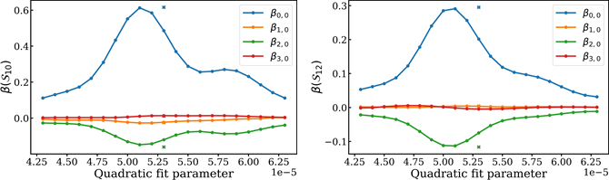
Fig. 4. Similar plots for the anisotropy parameters for sidebands 10 and 12 are shown. There is less sensitivity with a quadratic fit, and the sidebands are correlated with each other.

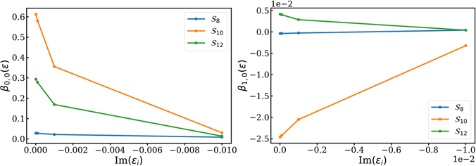
Fig. 5. Results for complex virtual orbital energies. The anisotropy parameters for ℓ = 0, 1 are shown for all sidebands. The anisotropy parameters all approach zero with increasing (negative) imaginary component.

In conclusion, PECD signals at RABBITT sidebands are sensitive to virtual orbital energies, sensitivity is present in anisotropy parameters, and imaginary parts can be added to virtual orbital energies to damp anisotropy parameters. In future work, we plan to switch to a higher level quantum chemistry calculation for more accurate results, and we hope to be able to match experimental results.

Acknowledgements
This project was done as part of the NSF Research Experience for Undergraduates at Kansas State University. I would like to acknowledge the KSU staff responsible for the program (Kim Coy, Loren Greenman, and JT Laverty) as well as my fellow undergraduate researchers. This material is based upon work supported by the National Science Foundation under Grant No. #2244539. Any opinions, findings, and conclusions or recommendations expressed in this material are those of the author(s) and do not necessarily reflect the views of the National Science Foundation. Computations for this project were performed on Beocat Research Cluster at Kansas State University, and used resources of the National Energy Research Scientific Computing Center (NERSC).

References
[1] R. E. Goetz, C. P. Koch, and L. Greenman, Phys. Rev. Lett. 122, 013204 (2019).

[2] F. A. Gianturco, R. R. Lucchese, and N. Sanna, J. Chem. Phys. 100, 6464 (1994).

[3] A. P. P. Natalense and R. R. Lucchese, J. Chem. Phys. 111, 5344 (1999).

[4] R. E. Goetz, C. P. Koch, and L. Greenman, arXiv: 2104.07522 (2021).

 

Final Presentation