For ultrafast laser pulse experiments, measuring the pulse width of the laser pulses is important. Pump-probe experiments use ultrafast laser pulses to create molecular movies of photo-induced molecular reactions. One of the laser pulses, the pump, starts the molecular reaction, and the second laser pulse, the probe, essentially images the reaction at a certain time interval from the pump pulse. Knowing the pulse width of the pulses helps determine the type of photo-induced reaction that can be imaged by providing a sort of “shutter speed” to the probe pulse. For example, if the pulse width is 100 fs, then it will not be able to image a reaction that takes 50 fs.

One method for measuring pulse width is an autocorrelator [1]. An autocorrelator has limitations when it comes to measuring pulse width because it requires an assumption of the pulse shape, always results in a symmetric autocorrelation even for asymmetric pulses, and cannot detect chirp [2]. A pulse is chirped when the wavelength of the pulse is time-dependent [3]. A pulse can become chirped whenever it travels through a medium since different wavelengths travel at different speeds. It is important to detect whether pulses are chirped.

For our setup, the autocorrelator was also limited by laser fluctuations which made it difficult to differentiate between noise and the actual signal. However, autocorrelators are useful because they can be used for virtually any wavelength of light, unlike other methods. Because of its relatively simple setup, it is also easier to diagnose problems since it is easy to access every part of it. My project focused on using an autocorrelator to measure the pulse width of the femtosecond laser pulses, and in the process, we discovered a method of identifying chirp in the pulses.

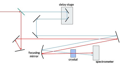
The setup for an autocorrelator is shown in Fig. 1. An incoming laser beam is split into two paths. The weaker, probe, laser path is shown in red and has a fixed length. Meanwhile, the stronger, pump, laser path length can be adjusted used a delay stage and is shown in blue. A spectrometer is used to collect the data from the probe laser. When the two lasers are not perfectly temporally and spatially overlapped inside the crystal, the spectrometer only measures the probe after one-photon absorption occurs in the crystal. When both lasers are perfectly overlapped, what’s known as time zero, two-photon absorption occurs inside the crystal, and more of the probe is used up, so the spectrometer measures the depletion of the probe beam.

Finding time zero was often the most difficult part of the experiment. First, we would have to make sure the two beams were focusing inside the crystal properly by aligning all the optics and moving the crystal back and forth. Then, we would move the delay stage until we saw a dip in the spectrometer which indicated we had found time zero.

We would take multiple loop scans by moving the delay stage which adjusted the temporal overlap of the two beams. The scans were taken before time zero, at time zero, and after time zero for multiple loops. We were taking spectrometer data as a function of delay. Using the spectrometer data, the pulse width can be calculated. The area or peak of each spectrum as a function of delay was plotted and fit to a Gaussian. To compute the pulse width, the full width at half max of the Gaussian fit was divided by two.

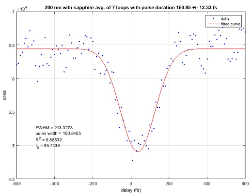
To test the autocorrelator, we used the laser from the OPA in the FLAME lab and the laser in the PULSAR lab. In PULSAR, we were able to measure a pulse width of about 150.85 +/- 13.33 fs for a 200 nm beam (see Fig. 2) which is relatively close to the expected measurement of about 140 fs from previous pulse width measurements. However, we were limited in our measurement because of fluctuations in the laser.

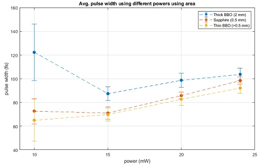
In FLAME, we compared the effect of using different crystals on the pulse width (see Fig. 3). We used a thick BBO crystal that had a thickness of 2 mm, a sapphire crystal with a thickness of 0.5 mm, and a thin BBO crystal that was even thinner than the sapphire crystal. The thicker the crystal, the greater the pulse width calculated, which makes sense because the pulse will stretch out as it travels through any medium, and a thicker crystal means there’s more medium to travel through. There is also a trend upward with greater input beam power which may be from saturating the crystal.

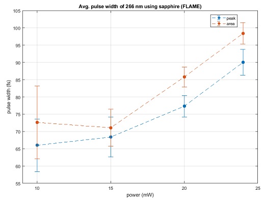
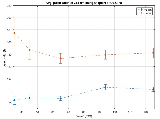
We also wanted to compare using the area with background subtraction of the spectrum versus the peak of the spectrum to find the pulse width. Theoretically, either method should yield the same pulse width. Figure 4 shows the comparison from the FLAME lab data, and it looks like the area measurement is larger than the peak measurement by about 10 fs. Figure 5 shows the comparison from the PULSAR lab data, and it looks like the area measurement is larger by about 50 to 100 fs. This huge discrepancy in the PULSAR data reveals that the area must be decreasing before the peak decreases before time zero, and then the peak increases before the area increases after time zero. This could be evidence of a chirped pulse.

The difference in the area and peak measurements is an indication of chirp because for an un-chirped pulse the peak and area deplete at the same rate as the two pulses overlap temporally. For a chirped pulse, the faster wavelength will deplete some of the area, then both the peak and area when most of the wavelengths overlap, and then just the area again as the slower wavelength arrives. We saw this behavior in our spectrometer data by creating an animation of the spectrum as a function of the delay (see Fig. 6). In Fig. 6, the faster, higher wavelengths arrive depleting just the right side, then the central peak depletes, and finally, the slower wavelengths arrive depleting just the left side.

We also plotted a 2D spectrogram which is shown in Fig. 7. For each delay, the spectrum is plotted as a vertical line with the color showing the amplitude to see the wavelength dependence of the depletion. The upper plot is the PULSAR data, and the lower plot is the FLAME data. It appears that the PULSAR data has a larger diagonal slope than the FLAME data which indicates the PULSAR pulses are more chirped than the FLAME pulses, and it explains why the area vs. peak pulse width calculations have a greater difference for PULSAR than for FLAME. The 2D spectrograms serve as a useful tool for identifying chirp in pulses from autocorrelator data.

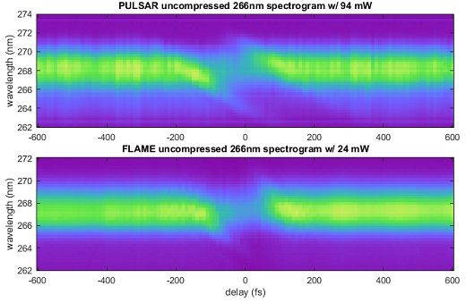
While the autocorrelator has limitations for measuring pulse width, it is a promising tool because of its broadband capability and relatively simple design. It appears it can also be used for chirp diagnosis in pulses, and other publications have shown the capability of retrieving a FROG trace from autocorrelator data [4]. In the future, implementing more background subtraction methods like a second reference spectrometer or chopper could greatly improve the pulse width calculations.

References

[1] Homann, C., Krebs, N. & Riedle, E. Convenient pulse length measurement of sub-20-fs pulses down to the deep UV via two-photon absorption in bulk material. Appl. Phys. B 104, 783 (2011). https://doi.org/10.1007/s00340-011-4683-0
[2] Paschotta, Rudiger. Autocorrelators. RP Photonics. https://www.rp-photonics.com/autocorrelators.html
[3] Paschotta, Rudiger. Chirp. RP Photonics. https://www.rp-photonics.com/chirp.html
[4] K. Ogawa and M. D. Pelusi. High-sensitivity pulse spectrogram measurement using two-photon absorption in a semiconductor at 1.5-µm wavelength. Opt. Express 7, 135-140 (2000). https://doi.org/10.1364/OE.7.000135

Acknowledgments

I’d like to thank my advisor Dr. Daniel Rolles as well as Surjendu Bhattacharyya, Zane Phelps, and Anbu Venkatachalam, for without their guidance and support this project wouldn’t have been possible. I would also like to thank everyone who organized the REU program as well as the National Science Foundation for providing funding.

Final Presentation