Through the use of ultra-fast laser pulses, it is possible to resolve the movement and interaction of electrons during photoemission. Streaked photoemission spectra are generated by way of a streaking setup, in which a neutral atom is photo-ionized by an ultra-short extreme ultra-violet (XUV) pulse. The ionized electron then interacts with a phase-coherent infrared (IR) laser, which acts as a ''clock" for the system and energy shifts the photoelectron.

Fig 1. An illustration how different initial states of the atom result in a time delay in the photoemission spectrum. An electron with a higher initial energy (shown in purple) will interact with a different portion of the streaking pulse than an electron with lower energy (red) as a result of the delay between emission. This results in an energy shift that can be measured and converted to find the relative emission delay. Adapted from [1].

Fig 2. Least-squares fit of a sinusoidal function to the measure photoemission peaks for the n=1,2,3 states (red, green, blue, respectively) of helium as found by our ab initio calculation. The relative time delays shown on the lower right are extracted from the fits. τ_exp is the experimental delay found from [2].

By varying the delay τ between the centers of the XUV and IR pulses, some insight into the dynamics of photoemission can be gained; specifically, the delay between emission from different processes and energy levels, see Fig. 1 for an illustration of this process. By comparing ab initio, experimental, and single active electron (SAE) results, the origin of the time delay can be examined [1].

Table 1: Comparison of relative time delays for n=1 and n=2 photoemission as found by Ossiander, et al. [2] and from our ab initio calculation.

Over the summer, I was working on comparing the time delays from the ab initio model to the experimental and computational time delays presented by Ossiander, et al. in [2]. Finding good agreement with experiment in relative time delays between the n=1 (shake-down) and n=2 (shake-up) photoemission [2], we were encouraged to calculate proposed relative time delays between n=1 and n=3 shake-up ionization, as seen in Fig. 2. Calculated streaking spectra are shown in Fig. 3 before interpolation and in Fig. 4 after interpolation.

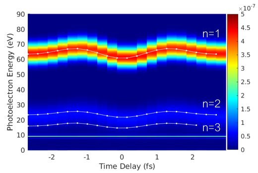
Fig 3. Streaking spectrum from our ab initio calculation. The white lines correspond to the n = 1 direct emission and n=2,3 shake-up ionization of helium, as labelled.

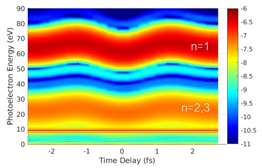
Fig 4. Interpolation of the spectrum shown in Fig. 3 with a logarithmic color scale. Direct and shake-up ionization are visible, but the n=2, n=3 shake-up ionization lines are overlapped.

I also worked on preparing for a comparison between the ab initio results and SAE results to help determine the source of the time delay. To this end, the final bound-state wavefunction was multipole expanded and the contributions to the effective time-dependent potential was calculated. Running SAE calculations without contributions from various multipole terms can point to the origin of the time delays, and can thus help to explain what time delays to expect from higher order shake-up ionization. Figure 5 shows the dipole term of the multipole expansion of the final state bound wavefunction at one instance in time.

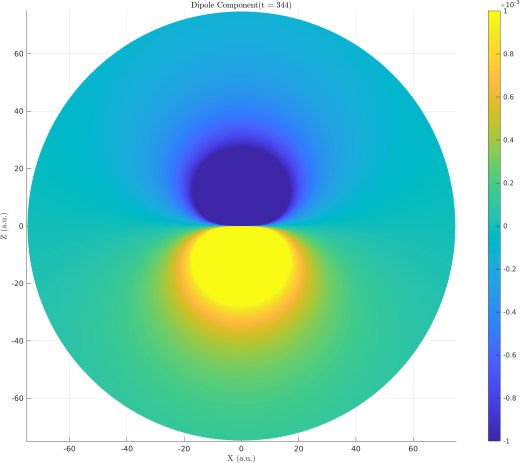
Fig 5. Dipole term of the multipole expansion of the final state bound wavefunction at t = 344 a.u. from the ab initio calculation.

References

[1] U. Thumm, Q. Liao, E. M. Bothschafter, F. Susmann, M. F. Kling, and R. Kienberger, Fundamentals of Photonics and Physics, Vol. 1 (Wiley, 2015) Chap. 13.

[2] M. Ossiander, F. Siegrist, S. V., R. Pazourek, A. Sommer, T. Latka, A. Guggenmos, S. Nagele, J. Feist, J. Burgdorfer, R. Kienberger, and M. Schultze, Nature Phys, 280 (2017)

Acknowledgments

I would like to thank Dr. Uwe Thumm for being my mentor on this project for the summer and Hongyu Shi for helping me immensely and putting up with my incessant questions. I would also like to extend my sincere thanks to Dr. Bret Flanders, Dr. Loren Greenman and Kim Coy for making this possible. This work was supported under NSF grant no. 1757778 and is part of an ongoing research project at the JRM Laboratory supported by the Chemical Sciences, Geosciences, and Biosciences Division, Office of Basic Energy Sciences, Office of Science, U.S. Department of Energy under award no. DEFG02-86ER13491.

Final Presentation