Particle Identification Away from the Bragg Peak Using dE/dx

Isabella Ginnett, Michigan State University, Physics and Mathematics Major

Mentored by Dr. Tim Bolton and Dr. Glenn Horton-Smith

MicroBooNE is a liquid argon time projection chamber (LArTPC) experiment that aims to further probe the low energy excess discovered by MiniBooNE [1]. To do this, MicroBooNE needs an array of excellent particle identification (PID) techniques. Traditionally, LArTPC experiments have relied on using dE/dx data around the Bragg peak of a particle's track. The reasoning behind this is that the separation in the average dE/dx of different particles is at its greatest there. Therefore, when this method works, it is quite effective. Figure 1 further illustrates why.

Figure 1. Plot of dE/dx versus the residual range for different types of particles as simulated by Geant4 [2].

However, there are several reasons why this method can break down. One reason is that particles do not need to be confined to the volume of the detector, meaning that the particle could leave the detector before its Bragg peak is reached. Also, particles do not strictly lose energy to ionization, the energy loss mechanism assumed by the Bragg peak method. This can lead to sharp deviations from the standard distribution of energy losses and an indistinct Bragg peak. Therefore, there is motivation to create new PID techniques that can still use dE/dx data but do not solely rely on the Bragg peak.

Although the difference in energy losses of different particles decreases farther away from the Bragg peak, the difference is still significant. Figure 2 illustrates this.

Figure 2. Plot of the Bethe equation, the formula that describes the average energy loss to ionization and electron shell interactions [3]. Specific portions of the curve are labeled to illustrate where a particle with those initial conditions would fall on the Bethe equation’s curve.

Additionally, proton momenta rarely exceed 1 GeV/c in MicroBooNE, and muons almost always behave like minimum ionizing particles in MicroBooNE. Therefore, the difference in dE/dx is even more significant for the particles created in the MicroBooNE detector, and data towards the middle of a particle's track can be used to differentiate minimum ionizing particles (MIPs) from highly ionizing particles (HIPs).

The technique works by selecting ten dE/dx points from the very center of a particle's track. From there, the truncated mean of those ten points is calculated. In essence, the truncated mean is just an arithmetic mean with outliers removed, and using this is important because dE/dx follows a highly skewed Landau-Vavilov distribution [4]. Then, the truncated mean is compared to MIP data using a χ² test. The reasoning behind this is that the MicroBooNE detector is well-calibrated to MIP data [5], so MIPs serve as a nice point of comparison. A schematic of how my algorithm works along with the χ² test formula can be seen in Figure 3.

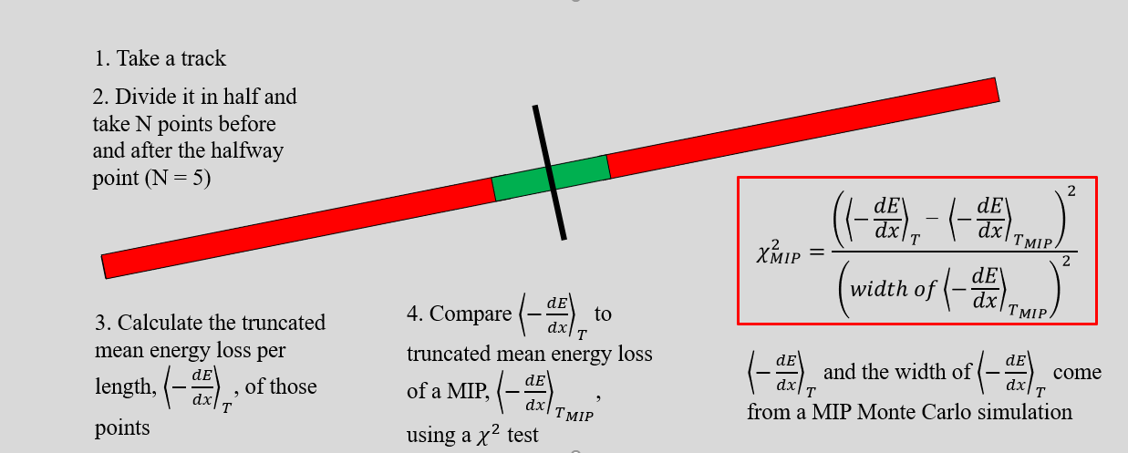
Figure 3. A schematic of how my algorithm works along with the formula used to calculate (χ² MIP) in the PID algorithm. <-dE/dx>T MIP and (width of <-dE/dx>T MIP) are calculated using simulated MIP data, or MC-Truth muon data where the initial momentum is 400 MeV/c.

I tested the performance of the algorithm on two MC-Truth data sets, one with 800 muons with an initial momentum of 400 MeV/c and one with 800 protons with an initial momentum of 1.2 GeV/c. The simulation itself relied on using software from DUNE [6], specifically dunetpc. The specific initial momenta were chosen in order to ensure that the track lengths of the muons and protons were around 130 cm. Figure 4 histograms the distribution of (χ² MIP) for both the muon and proton samples.

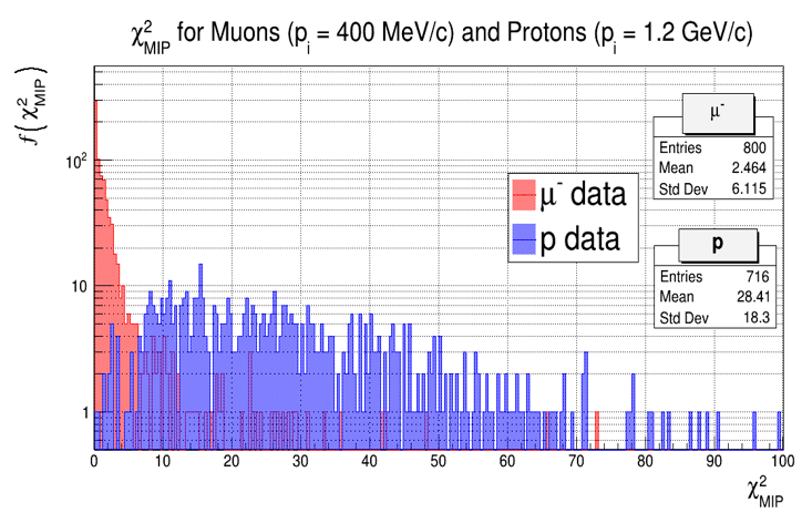
Figure 4. Histogram that plots (χ² MIP) for both muons and protons. The muon sample contained 800 particles that had an initial momentum of 400 MeV/c. The proton sample contained 800 particles that had an initial momentum of around 1.2 GeV/c.

Figure 4 nicely illustrates how there is great separation between the muon (χ² MIP) distribution and the proton (χ² MIP) distribution, indicating that my algorithm identifies particles effectively.

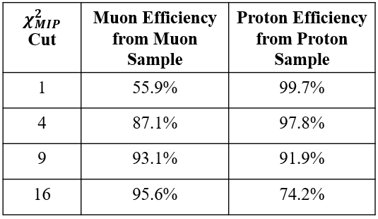
In order to identify the particle, there needs to be some sort of cut on (χ² MIP). If (χ² MIP) < (χ² MIP Cut), then the particle is a MIP. If (χ²) MIP > (χ² MIP Cut) then the particle is a HIP. I tested different (χ² MIP) cut values to see how the efficiency of the algorithm would change. Table 1 illustrates those results.

Table I: Table that displays how the (χ² MIP Cut) impacts the efficiency of the algorithm's PID.

In summary, particle identification techniques away from the Bragg peak are quite useful, and using the truncated mean dE/dx in the middle of a particle's track shows great promise as a means of doing this. Looking into the future, I would like to investigate how the algorithm behaves at different test track lengths to better understand where this method would be the most effective.

References

[1] https://microboone.fnal.gov/

[2] The MicroBooNE Collaboration, "Selection of ν_μ charged-current induced interactions with N>0 protons and performance of events with N=2 protons in the final state in the MicroBooNE detector from the BNB," MICROBOONE-NOTE-1056-PUB (2018).

[3] M. Tanabashi et al. (Particle Data Group), Phys. Rev. D 98, 030001 (2018).

[4] For more information on the Landau-Vavilov distribution, see the following link: http://meroli.web.cern.ch/Lecture_landau_ionizing_particle.html

[5] The MicroBooNE Collaboration, "Detector calibration using through going and stopping muons in the MicroBooNE LArTPC," MICROBOONE-NOTE-1048-PUB (2018).

[6] https://www.fnal.gov/pub/science/lbnf-dune/index.html

Acknowledgments

I would like to thank Dr. Tim Bolton and Dr. Glenn Horton-Smith for the guidance they have provided all throughout the summer. I would also like to thank Harry Mayrhofer and Norman Martinez for their help and support as well. Additionally, I would like to thank the MicroBooNE Collaboration and the DUNE collaboration for providing data and software, Dr. Bret Flanders and Dr. Loren Greenman for organizing the REU, Kansas State University for hosting the REU, and the National Science Foundation for funding.

Final Presentation