Median Statistics Analysis of Deuterium Abundance Measurements and Spatial Curvature Constraints
Jarred Penton
Fort Hays State University
Physics Major
Mentored by Dr. Bharat Ratra
We analyzed a dataset compiled by Zavarygin et al. (2018), hereafter Z18, that included deuterium abundance measurements.
Table 1. D/H measurements from Z18.
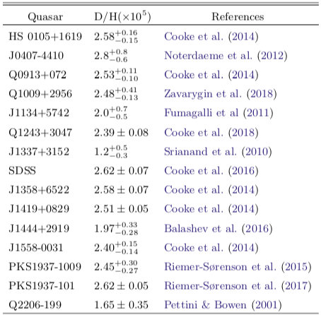
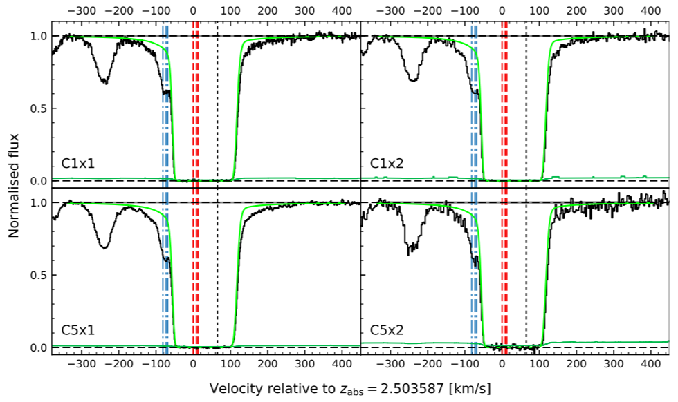
Figure 1. Spectroscopic analysis data collected by Zavarygin et al. (2018). The blue lines indicate deuterium absorption and the red line indicates hydrogen absorption
With 15 different measurements, Z18 determined that two outliers (Srianand et al. 2010 and Pettini & Bowen 2001) should not be included in the data set then determined a weighted mean central estimate. We recreated this analysis as well as performed our own analysis on the full data set. Using the Kolmogorov-Smirnov Test, we analyzed the gaussianity of the two data sets (Truncated 13 and All 15).
Table 2. KS Test Probabilities a: The scale factor S fixed to 1 or that which maximizes p. b: The probability (p-value) that the data doesn’t not come from the PDF. c: Student’s t distribution parameter n.
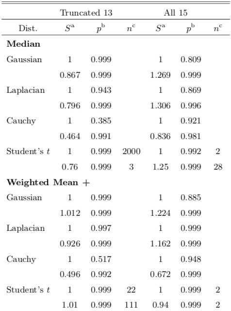
Table 2 shows analysis on four separate error distributions drawn from different central estimates. The p-value shows the percent likelihood that our distributions didn't not come from the distributions we are testing against (in this case: Gaussian, Laplacian, Cauchy, and Student's t). It is clear that the Truncated 13 data set is gaussian and the All 15 data set is non-gaussian. We decided that a median statistics approach to analysis is appropriate when determining a central estimate for the All 15 data set. We found that the Truncated 13 weighted mean central estimate is (D/H)p = (2.544 +/- 0.025)x10-5 (slightly different than Z18's 2.545 measurement), and the All 15 median central estimate is (D/H)p = (2.48 +/- 0.065)x10-5 with a symmetrized error. Using these central estimates, we use an equation from Coc et al. (2015)
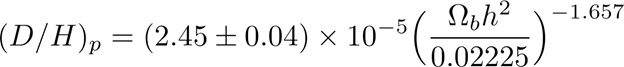
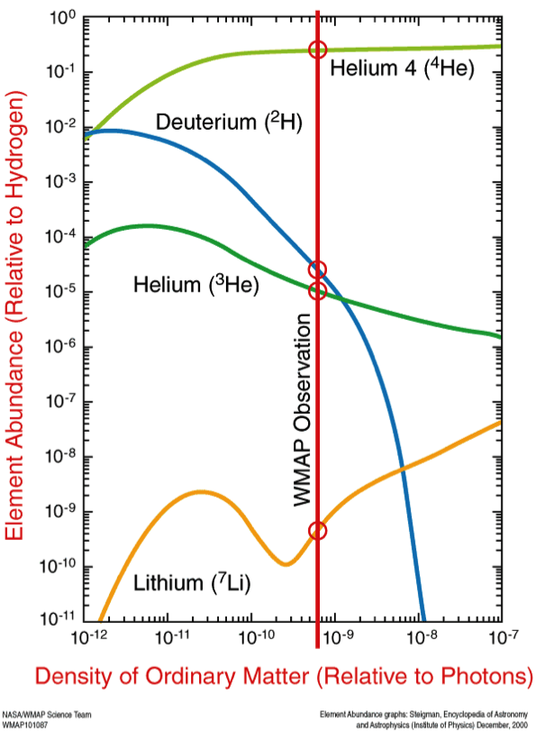
Figure 2. Shows the correlation between abundance of light elements (y-axis) and the baryonic density of the universe (x-axis) as well as a current CMB prediction on the baryonic density (red vertical line)
For the weighted mean central estimate Ωbh2 = 0.02175 +/- 0.00025, and for the median central estimate Ωbh2 = 0.02209 +/- 0.00041. We compared these two values to Ωbh2 's determined using other cosmological data and cosmogonical models, and found by how many standard deviations, σ, they differ.
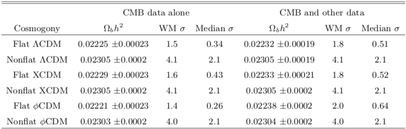
Table 3 shows three different CMB models, each with a flat universe and nonflat universe variant, as well as these same models in addition to other cosmological data and their corresponding value for Ωbh2 .
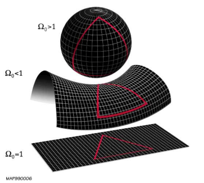
In conclusion, the median statistics central estimate (D/H)p-determined Ωbh2 is more consistent with the cosmologically-determined Ωbh2 's than the weighted mean central estimate Ωbh2 . In both cases, it seems (D/H)p-determined Ωbh2 's favor flat universe predictions over nonflat predictions.
References:
Balashev, S. A., Zavarygin, E. O., Ivanchik, A. V., Telikova, K. N., & Varshalovich, D. A. 2016, MNRAS, 458, 2188 [arXiv:1511.01797]
Coc, A., Petitjean, P., Uzan, J.-P., et al. 2015, Phys. Rev. D, 92, 123526 [arXiv:1511.03843]
Cooke, R. J., Pettini, M., Jorgenson, R. A., Murphy, M. T., & Steidel, C. C. 2014, ApJ, 781, 31 [arXiv:1308.3200]
Cooke, R. J., Pettini, M., Nollett, K. M., & Jorgenson, R. 2016, ApJ, 830, 148 [arXiv:1607.003900]
Cooke, R. J., Pettini, M., & Steidel, C. C. 2018, ApJ, 855, 102 [arXiv:1710.11129]
Fumagalli, M., O'Meara, J. M., & Prochaska, J. X. 2011, Science, 334, 1245 [arXiv:1111.2334]
Noterdaeme, P., Lopez, S., Dumont, V., et al. 2012, A&A, 542, L33 [arXiv:1205.3777]
Pettini, M., & Bowen, D. V. 2001, ApJ, 560, 41 [arXiv:astro-ph/0104474]
Riemer-Sørensen, S., Webb, J. K., & Crighton, N., et al. 2015, MNRAS, 447, 2925 [arXiv:1412.4043]
Riemer-Sørensen, S., Kotus, S., Webb, J. K., et al. 2017, MNRAS, 468, 3239 [arXiv:1703.66656] S
rianand, R., Gupta, N., Petitjean, P., Noterdaeme, P., & Ledoux, C. 2010, MNRAS, 405, 1888 [arXiv:1002.4620]
Zavarygin, E. O., Webb, J. K., Dumont, V., & Riemer-Sørensen, S. 2018, MNRAS, 477, 5536 [arXiv:1706.09512]