Simulating 1-Dimensional Amyloid Copolymerization

Noeloikeau Charlot

University of Hawaii at Manoa

Physics, Biological Engineering Major

Mentored by Dr. Jeremy Schmit and Dr. Chris Sorensen

The objective of this project is to simulate a one-dimensional amyloid copolymer consisting of two subunits: IAPP (amylin) and Aβ (amyloid beta). IAPP is secreted alongside insulin and has been linked to type-II diabetes. Aβ is the main component of amyloid plaques associated with Alzheimer's.

This project builds on work done by Sheena Radford (2017) on IAPP/Aβ amyloid copolymerization, and explores the case in which binding between dissimilar subunits is stronger than binding between similar subunits. Changes in chain constituency and growth rate are modeled as a result of altering monomer concentration, ratios, and binding energy. This work helps to address our limited understanding of amyloid copolymers, with applications in medicine and materials science.

The simulation consists of a modified Gillespie algorithm which randomizes addition and subtraction of monomers to the end of the chain, obeying certain thermodynamic constraints. For instance, the subtraction of the most recent element added to the chain is inversely proportional to the exponential of the binding energy.

The system can be simplified to two molecules, denoted A & B. These molecules form a linear chain which may consist of an Alternating, Block, or Random sequence. The type depends on the binding energy E between adjacent molecules. If we let I denote the last position in the chain, the possible reactions are

I→IA (Eq. 1)

I→IB (Eq. 2)

I→(I-1) (Eq. 3)

i.e A can be added, B can be added, or the last element removed. If we let K₁ be the reaction rate for addition of A, K₂ be reaction rate for addition of B, K₃ ∝ exp(-E) be the reaction rate for last element removal, and K_tot= K₁+K₂+K₃, then the simulation consists of the routine:

1) Generate random number: 0<R₁<1

2) If: { R₁≤K₁/K_tot : add A to chain ; R₁≤(K₁+K₂)/K_tot : add B ; else remove }

3) Generate random number: 0<R₂<1

4) Update timestep defined by: t+= -ln(1-R₂)/K_tot

5) Repeat

Within the execution of this routine, various parameters are calculated, most notably the order parameter M = (1/L)∑_si from i=1 to i=L where s = {-1: A; +1: B} and L = length of chain, which can be thought of as the composition of the aggregate amyloid chain. Additionally we define the growth rate G = L/t.

The outputs of the simulation are the values of M and G at various values of the concentration of monomers C, the binding energy E, and the ratio of monomers A to B given as P, which can be thought of as the composition of the amyloid monomers in the solution.

These results are shown below:

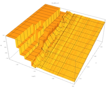
Fig. 1: (C,P,M) surface at E=1. At both high and low concentrations M~P, indicating a linear relation.

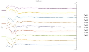
Fig. 2: (C,M) level sets of P at E=1. Same data as Fig. 1, highlighting linear relation with statistical deviations at low C.

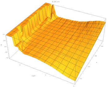
Fig. 3: (C,P,M) surface at E=5. At high concentrations M~P, but at low concentrations M~constant, indicating a sigmoidal relation.

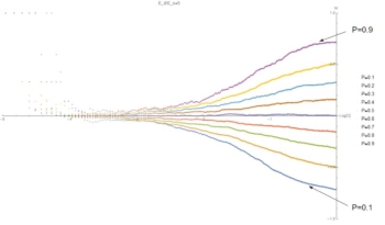
Fig. 4: (C,M) level sets of P at E=5. Same data as Fig. 3, highlighting sigmoidal relation.

These graphics show that for small E the relation between composition of the aggregate ("M") and composition of the solution ("P") is independent of concentration and linear with P. At large E, and for low concentrations, M is constant. At high concentrations, M depends on P. This indicates a sigmoidal relation.

Now, we turn to the growth rate G.

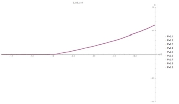
Fig. 5: (C,G) curve at E=1. Symmetry causes G to be independent of P as the particles are indistinguishable.

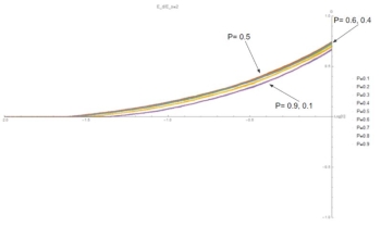
Fig. 6: (C,G) curves at E=2. Symmetry is broken and G is no longer independent of P. Values of P closest to 0.5 show the highest growth rate because the chain alternates between A and B, maximizing the number of strong bonds and minimizing the number of off events.

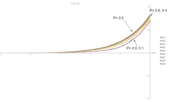
Fig. 7: (C,G) curves at E=5. As E increases, G becomes nonzero at lower values of C. This is because at low concentrations the binding energy allows bonds between different types to persist in the time between addition events.

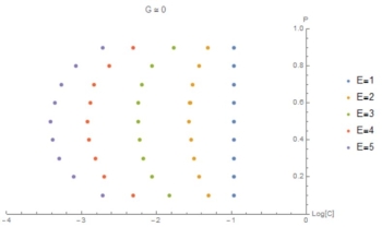
Fig. 8: (C,P) curves at the point G=0. This graphic highlights the previous result that as E increases G becomes nonzero at lower values of C.

In summary, at high concentrations the composition of the aggregate is determined by the composition of the solution, while at low concentrations the composition of the aggregate is determined by binding energy. Furthermore, chains with high binding energies begin growing at lower concentrations. Further research could account for different monomer masses, charges, and structures.

Acknowledgments

The author would like to acknowledge Kansas State University Research Opportunity for Undergraduates and the National Science Foundation for funding and research equipment, as well as Dr. Jeremy Schmit and Dr. Chris Sorensen for research advice and direction.

 

Final Presentation