Pump-probe spectroscopy is one experimental method for measuring nuclear vibrational dynamics, and consists primarily of a three step process:
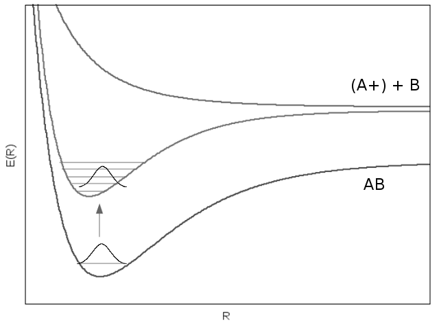
Beginning with a neutral molecule in its ground state, a laser pulse (the probe pulse) induces an electronic transition to an excited molecular orbital. In the excited state, the post-transition wavefunction is composed of a superposition of stationary-state wavefunctions corresponding to vibrational energy levels.
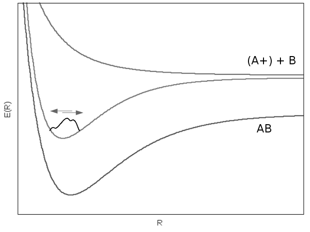
After the pump pulse, the excited molecule is allowed to oscillate in its excited state for a particular delay time. Due to the the anharmonicity of molecular potential wells, vibrational energy level stationary state wavefuncitons oscillate at different frequencies, which causes dephasing through interference. After some amount of time (related to the geometric properties of the specific orbital’s molecular potential curve) the entire wavefunction comes back into phase and so-called “vibrational revival” occurs.
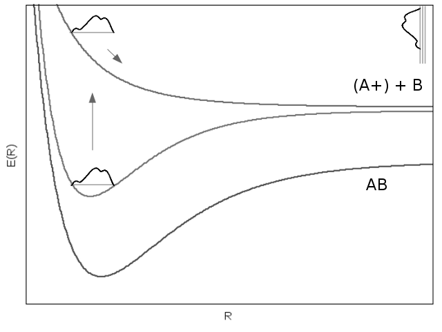
After field-free oscillation for a certain delay time \(\tau\), a second laser pulse, termed the probe pulse, can be used to induce an electronic transition to either a dissociative molecular orbital or a \(\frac{1}{R}\) Coulomb repulsion curve. Either way, the molecule dissociates, and ion fragments can be measured using techniques such as velocity map imaging. Repeating this experiment across a spectrum of delay times can be used to model the time evolution of the wavefunction through the ion fragment energy release spectrum.
As mentioned above, an electronic transition to an excited molecular orbital results in a wavefunction composed of contributions from various stationary-state eigenfunctions corresponding to each vibrational energy level in the excited state. As the excited wavepacket evolves in time, phase interference between these stationary-state wavefunctions causes the overall wavepacket to dephase. Eventually, the wavefunction comes back into phase. This is termed a vibrational revival, and the periodic nature of these revivals can give information on how the overall molecular wavefunction (and hence the nuclear motion of the molecules) evolves in time.
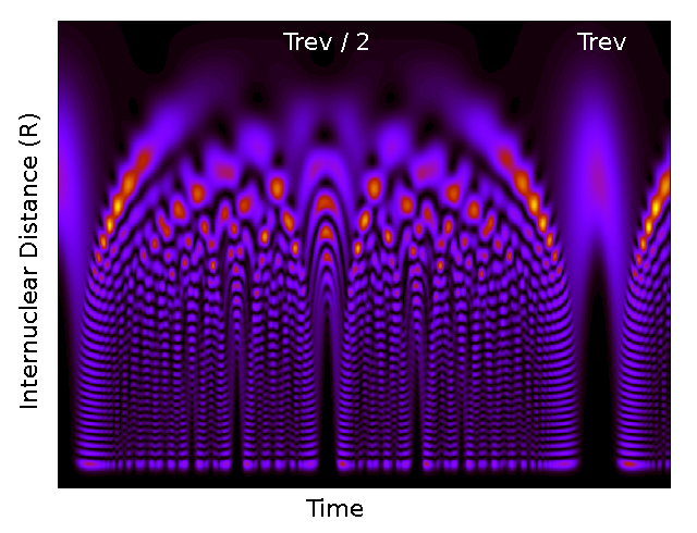
The picture below displays an example of how \(\left|\Psi \right|^2\) evolves in time. The periodicity of its time evolution along with the the full, and half vibrational revivals can be clearly seen.
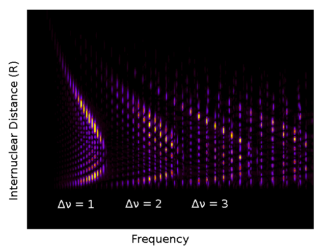
By Fourier transforming the time evolution of the wavefunction, the beat frequencies of the oscillatory motion of vibrational energy level wavefunctions can be seen. An example is shown below. Since these vibrational wavefunctions oscillate at different frequencies, their oscillations beat against each other. Identifying characteristic beat frequencies in power spectra calculations can be used to identify between contributing vibrational energy levels (and even between contributing electronic states in more complicated situations), identify structural characteristics of vibrational energy levels, and map out derivatives molecular potential curves.