H₂O

Experiment Description

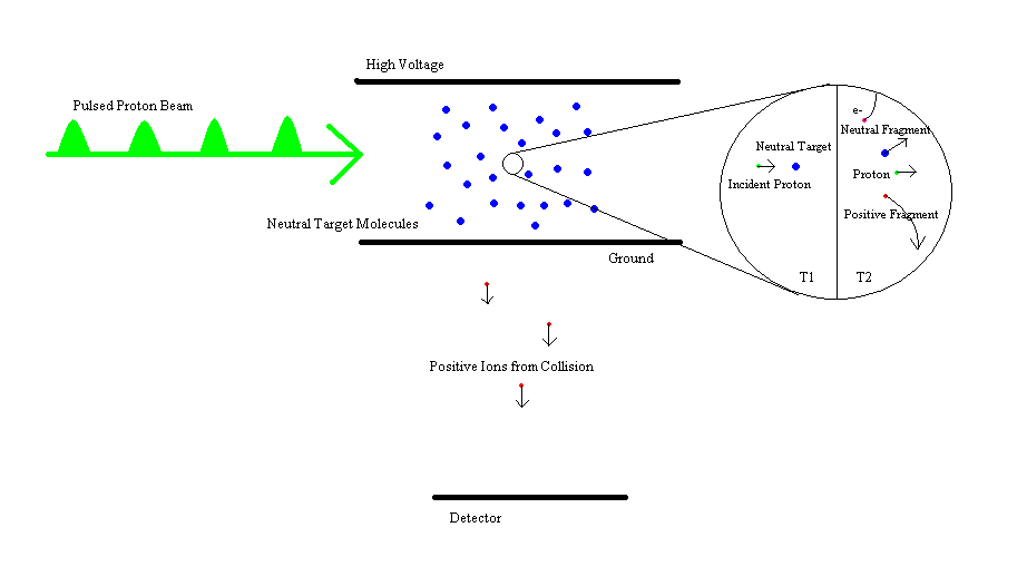
Protons are accelerated in pulses and collide with "stationary" H2O molecules. The interaction takes place inside a region of elevated electric potential, so charge particles are accelerated to a detector. The energy of the protons can be controlled, as can the composition of the target. Specifically, we will be examining runs with 4 and 1 MeV protons colliding with H2O, D2O, and HDO. A basic schematic of the design can be found below.

(Note: Not to scale.)

When the proton collides with the neutral target, a number of things can happen. The neutral target could remain intact, it could disassociate, or it could ionize. Any positively charged particles are accelerated out of the interaction region to the detector. (After the interaction, the protons still have a great enough kinetic energy that they travel out of the interaction region without being detected.) At the detector, the time of flight is measured using the timing of the proton pulses. It can be shown that the time of flight is proportional to sqrt(mass/charge) of the positively charge fragments. This is intuitive since one would expect massive particles to be accelerated more slowly and thus have a greater time of flight than lighter particles. The inverse can be said of highly charge particles compared to low charge particles.

Corrections

This method of particle detection is useful, but it has some limitations. For instance, the detector cannot distinguish between two particles of identical mass and charge, or two hits involving two particles of the same mass/charge ratio. Thus, in our system, we cannot initially distinguish between H2(+) and D(+), or the Hydrogen ions in the H2O → H(+) + H(+) + O(+) reaction. Furthermore, the detector efficiency is only about 35%, so sometimes events occur without being detected, or only a fraction of the particles involved are detected. Also, more than one reaction can occur in the same pulse, so random coincidences appear. In the random coincidences case, for instance, we might detected an O(+) and an OH(+). Clearly, these fragments are not the result of an ionization and disassociation of O2H(+), they are the results of two distinct interactions. In that case, most likely we detected the O(+) from a H2O → H(+) + H(+) + O(+) interaction and the OH(+) from a H2O → H(+) + OH(+). We tackle these problems with perturbation theory.

In my explanation of our perturbation theory method, I will consider a different, less complicated target: HD. While it gets much more complicated with isotopic water, the same general idea applies. The possible reactions involving HD are:

HD → HD(+): Detect HD(+)

HD → H + D(+): Detect D(+)

HD → H(+) + D: Detect H(+)

HD → H(+) + D(+): Detect H(+) and D(+)

The calculation of the actual number of HD → HD(+) from the data is straight forward since it cannot be confused with the other reactions. However, the other reactions are coupled. When we detect an D(+) it could be from an HD → H + D(+) reaction or a HD → H(+) + D(+) reaction in which we lost the H(+). Furthermore, when we detect an H(+) and a D(+), that could be a HD → H(+) + D(+) reaction or a random coincidence between a HD → H + D(+) reaction and a HD → H(+) + D reaction. Thus, we arrive the following equations, where M(x) the measured counts of a species x and N(x) is the actual number of counts of a species x:

Let ε be the detector efficiency and τ be the likelihood of a random coincidence.

M[HD(+)] = εN[HD(+)]

M[H(+)] = εN[H(+) + D] + N[H(+) + D(+)]ε(1-ε)

M[D(+)] = εN[H + D(+)] + N[H(+) + D(+)]ε(1-ε)

M[H(+) + D(+)] = ε²N[H(+) + D(+)] + τN[H(+) + D]N[H + D(+)]

We then apply several iterations to the coupled equations with the first assumption being that τ = 0, since in reality τ is very small.

1st iteration:

M[H(+)] = εN₀[H(+) + D] + N₀[H(+) + D(+)]ε(1-ε)

M[D(+)] = εN₀[H + D(+)] + N₀[H(+) + D(+)]ε(1-ε)

M[H(+) + D(+)] = ε²N₀[H(+) + D(+)]

Solve for N₀[H(+) + D], N₀[H + D(+)], and N₀[H(+) + D(+)].

2nd iteration:

M[H(+)] = εN₁[H(+) + D] + N₁[H(+) + D(+)]ε(1-ε)

M[D(+)] = εN₁[H + D(+)] + N₁[H(+) + D(+)]ε(1-ε)

M[H(+) + D(+)] = ε²N₁[H(+) + D(+)] + τN₀[H(+) + D]N₀(H + D(+)]

Solve for N₁[H(+) + D], N₁[H + D(+)], and N₁[H(+) + D(+)].

3rd iteration:

M[H(+)] = εN₂[H(+) + D] + N₂[H(+) + D(+)]ε(1-ε)

M[D(+)] = εN₂[H + D(+)] + N₂[H(+) + D(+)]ε(1-ε)

M[H(+) + D(+)] = ε²N₂[H(+) + D(+)] + τN₁[H(+) + D]N₁(H + D(+)]

Solve for N₂[H(+) + D], N₂[H + D(+)], and N₂[H(+) + D(+)].

Repeat the process until the solutions stop changing. Again, with isotopic water, the process is much more complicated, but the same general approach applies.

Finally, contamination is present in the target and this contamination appears in the data. The contamination mainly consists of the other isotopic water molecules from previous runs, and N2(+) and O2(+) from the atmosphere. To remove the contamination from air, a run was conducted with only air. We decoupled the air data and then removed it from the samples by scaling the ratio of counts in a specific channel (i.e. m/q value, or values for pairs and triples) to the counts in the O2(+) channel. We performed a similar scaling procedure with removing the isotopic water contamination, but in a more precise iterative method.

Problems in Correction Process

Unfortunately, all did not go as planned in the correction process. We first examined the 4 MeV protons on isotopic water runs. H2O and D2O decoupled perfectly within Itzik's program, but HDO did not. From that point, we attempted two correction methods. First, we simply removed contamination from the data without decoupling and compared our results to previous analysis of the data by Max. This showed that while some purely coincidental channels remained within the data, on channels that were realistic, the data was very close to Max's previous analysis. Furthermore, the results of combining the coupled HDO file with the decoupled H2O and D2O data allowed for the iterative method to continue. This method produced results that are generally closer to Max's previous analysis. Since the coupled method appears to have worked just as well as decoupling, we applied the coupled method to the 1 MeV data. We have no check for the results of this method since the 1 MeV data defied decoupling in Max's previous analysis. We present some of our brief analysis of this 1 MeV data in the final presentation. Unfortunately, due to time constraints we were unable to include error.

Last Modified: 8-02-07