Week 1: 5/26-5/30

We listened to presentations for all of the projects available to REU students this summer. We picked our specific projects.

Once assigned to our projects, we had to read a lot of background information about our projects. We read the proposal for Double Chooz, the KamLAND projet Summary, the tutorial for Geant4, and Safety information about KamLAND itself. We also had several meetings in which we discussed the basic science behind the neutrino experiments.

Week 2: 6/2-6/6

We all had to learn about individual particles. I read up on alpha and beta particles, and how they interacted with the scintillator fluid. Then I gave a presentation about it.

We had to learn about C++ and how Geant4 works, so we were given toy programs. I was assigned studying the interactions that had to do with alpha and beta particles. I started on Beta particles, and began modeling what happened to an electron in a detector. That was very complex, but my mentor wanted me to mainly focus on the electron/positron annihilation; therefore, instead of starting with an electron, which could do a whole bunch of different things in the scintillator fluid, I instead started with a positron.

There are two types of electron/positron annihilations. I focused on the low energy annihilation. In this annihilation, the positron loses energy, and eventually loses enough energy that it begins to orbit an electron. The electron and positron form positronium. The two particles orbit each other and over time lose energy. Thus, the positronium collapses, and the two particles annihilate at rest, producing either two or three photons.

My mentor suggested I further simplify this situation. I should only model the case that two photons are created, traveling in opposite directions. Also, instead of trying to calculate the positron’s motion in orbit with the electron, I should just allow the positron to slow down until it stops, and once its velocity = 0, allow the positron to annihilate.

My program goals were this: have a user input the initial position and momentum of the positron. My program would then send the positron through the scintillator fluid. As the positron travelled, it would ionize the atoms in the scintillator fluid. This ionization requires energy from the positron, so as the positron ionizes the scintillator fluid, it loses energy and slows down. This is modeled by the Bethe-Bloch formula. Eventually the positron comes to a stop, and at that point I force annihilation. Basically, my program kept track of the position of annihilation, and from that spot emitted two photons travelling in opposite directions. An important point here is to make sure that the photons are randomly generated in such a way that if this process were to happen thousands of times (or my program was to run thousands of times), the distribution of the photons would be isotropic.

To explain the term isotropic, let’s assume that the positron annihilates in exactly the same spot thousands of times, each time producing two photons. Now, let’s construct a sphere around this spot where the positron annihilates (so that this spot is the center of the sphere). Every time the positron annihilates, two photons are produced, and travel radially outwards from the center of our sphere. Each photon passes through the sphere, and we will draw a little black dot on the sphere where the photon hit the surface of the sphere. After thousands of annihilations, there should also be thousands of corresponding dots on our sphere. These black dots could be grouped together in different ways. They could cluster near opposite poles of our sphere, or there could be a great concentration near an equator. We want these black dots to represent an isotropic distribution. This means that we want there to be an even distribution of dots on the entire surface area of the sphere.

So, now it was my job to randomly generate the photons in such a way that they would have an isotropic distribution. I had to generate one photon randomly, and have the other photon go in exactly the opposite direction as the first photon. I was correct in thinking this problem would be much easier to solve in spherical coordinates rather that Cartesian. A vector in spherical coordinates has two angles, which indicate direction, and one coordinate “r”, which indicates magnitude. Because my photons always annihilate at the same energy (because each annihilation has the same initial energy), r was fixed. Therefore, I only had two degrees of freedom: theta and phi.

Unfortunately, it’s not enough to just generate theta and phi randomly. When you do that, you don’t get an isotropic distribution, but you do get a crowding near the poles of the sphere. This is because of the nature of spherical coordinates. If you pick a fixed phi, and vary theta, the phi sweeps out a ring on our sphere. Now if you randomly generate phi, you get a set of rings on the sphere. If you randomly generate theta for each ring, you get the approximately the same number of hits on each ring of the sphere. So the ring around the equator gets about 1000 hits, spread out over the whole equator. Then the tiny ring near the pole get the same number of hits as the equator, and thus 1000 hits are crowded together in a tiny area. Then there are exactly 1000 hits on the spot at the pole where phi = 0. This isn’t an isotropic distribution, so this is a problem. So, how do we fix it? We randomly generate cos(phi). This causes an isotropic distribution, which can be showed by this histogram of my angle phi:

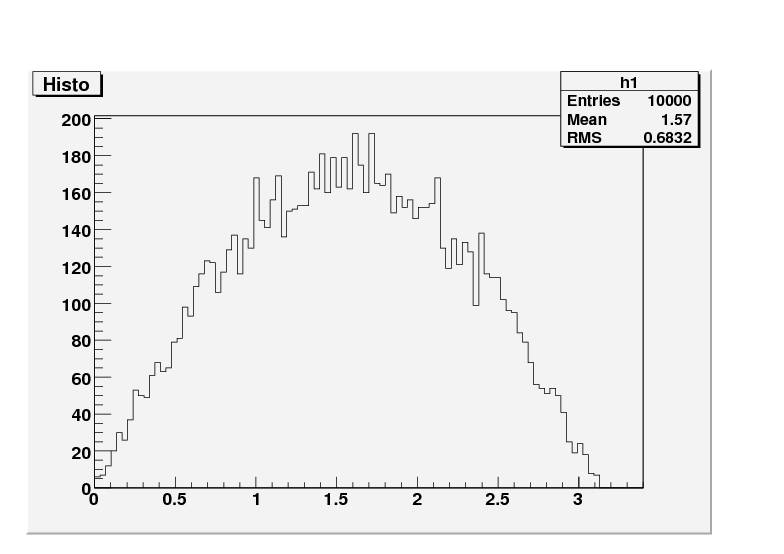
Notice how there are more hits around phi = pi/2. This means that more hits occur at the ring around the equator, and few hits occur on the rings near the poles. This histogram indicates an isotropic distribution of photon directions.

Week 3: 6/9-6/13

I worked most of the kinks out of my program. Also, we tried to install Dogs and Geant 4 onto our computers, but it was long and difficult. The tornado hit, so we couldn’t go into work. Then the power went out the next day in Cardwell, so we couldn’t really get any more work done. Instead, we learned about root and how to make histograms of the data we could find with our programs.

Week 4: 6/16-6/20

We learned how to install Geant4, and spent all day trying to get it installed on everyone’s computers, solving particular problems that came up with everyone. I finally fixed my program. It turns out the biggest problem was unit conversions. Once I got that all worked out, however, my program worked fine, and I was able to start making histograms of the output of my program. Also, we ran a macro to test our installation, lytest.mac, and then we modified the macro, and made an actual simulation.

This week we got our actual research projects. I chose to model the background radiation produced by the glass in the PMT’s. The PMT’s capture the light from the scintillator fluid, observing neutrino effects. The problem is that glass has some radioactive materials in it, namely, U238, Th232, and K40. With this model, we can be able to more correctly understand the background “noise” produced from the glass PMTs, and thus be able to subtract it out of the final measurement.

I spent a lot of the week reading papers that were done for KamLAND modeling similar things. Then we learned a little bit about writing macros.

Week 5: 6/23-6/27

I did more background reading, but despite reading about previous projects, I still could not understand exactly where to begin. Then the building got evacuated due to asbestos. While our mentors were away and the building was evacuated, we received lectures from Larry Weaver about the general science behind neutrinos, and the implications of observing neutrino oscillations.

On Wednesday, we went to Pillsbury Crossing and played in the river. There was no crowd, it was beautiful out, and I got to swim under the waterfall. It was a pretty awesome Wednesday.

Week 6: 6/30-7/4

I started generating a macro. I noticed that after my first 1000 events, my events were happening way too long. My mentor told me over email to get the rate of the events. I wasn’t sure how to do this, so I found a function to get the time of the event. I found out my events were taking way too long, but the first 1000 were fine. I didn’t understand this. Then I realized that because I had run two different macros, but not changed the names of the data file generated, the macro stored the information from two separate runs into the same folder. I finally realized that I had to move the files from my first run into a separate folder. Once I did that, however, I ran out of space on my hard drive. At this point I needed more space in order to store data from difference simulations. Also, now the 1000 events that happened in a reasonable time were removed, and I could only deal with the other events that took way too long.

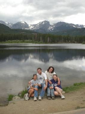
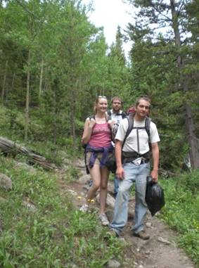
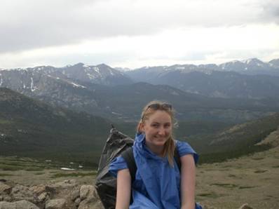
This weekend we went backpacking in the Rockies. It was really fun, but very hard work. By hard work, I mean the most physically demanding activity I’ve done in the last year. Yoga just doesn’t prepare you for a 20-mile trail loop, with backpacks, 12,000 feet up, racing against the thunderstorms to get to the next campsite. Seriously, though, I had lots of fun.

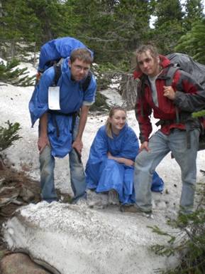
Yes, that is snow.

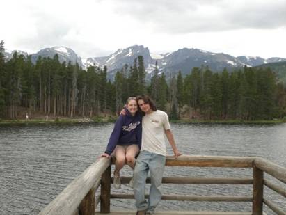
See those mountains in the background? There was a point where

we were higher than them. This was our climb down.

Week 7: 7/7-7/11

Using Geant4, I generated decay for Bi214. I wasn’t exactly clear on where I generated these events. Also, I noticed that my events happened at around 10^30-10^33 nanoseconds. This is way too long. I output the times of each event to a data file, so that I could understand why each event took so long to generate. When I asked Dr. Horton-Smith, he said I should ignore the extra-long timing. It’s a byproduct of the way the code was written.

My next task was to find and count all of the events that deposited energy above .5 MeV, .7MeV, and 1 MeV, for each of the four materials. Then I had to find and count all of the parent decays. I used a function to get the event type. If the event type is 3, it’s a parent decay. Events that are type 51 are not parent decays, but gammas. I then counted the events that were of type 3, and thus counted the parent decays.

I found the ratios by calculating events above a certain threshold, and dividing it by total parent events for Bi214. I then created macros that would do the same thing, only with U238, Th232, and K40. I found the ratios for all three thresholds and for all four elements. Then I compared the ratios I found to previous ratios.

Energy Deposition above zero for Th232 in both

the gamma catcher and the target:

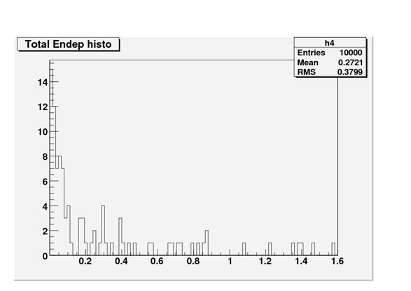
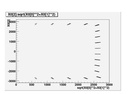
My ratios didn’t match at all. When I examined what could have gone so badly, I found that the parent decays were not occurring in the PMT glass, but in the buffer solution. I edited the macro with new coordinates for the PMTs. I figured out how to make a plot to see exactly where the parent events occurred, and thus give me a clear picture of the PMT’s. I only modeled a few PMT’s, and argued that symmetry would account for the rest.

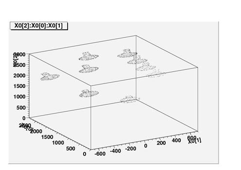
I found a better way to get the PMTs. I basically told Geant4 to start the events in the glass, instead of in specific PMTs. This was more accurate, and I got some results from that. Here’s where the parent events started in my new, better method:

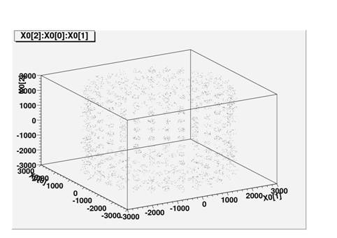
This shows all of the PMT’s in the buffer being site of parent decay.

Week 8: 7/14-7/18

I get error bars for my data, and found that the data was still too far off. My data did have a trend of being generally below what was expected from previous results.

Now I have to find the attenuation. If I find how many of the photons in the back of the PMT’s didn’t make it to the front, it might be a good explanation for why my data is off. I also want to start filling the area that will be filled with sand. Glenn said to fill the Inner Veto Shielding Wall with my events. I don’t know how to write this in a macro, but I can try.

Week 9: 7/21-7/25

I wrote the macro to fill just the steel in the Inner Veto. This was extremely difficult, and I couldn’t make it work the first twenty times I tried.

These are bad pictures. It looks like on this try, I filled steel that is attached to the PMT’s, and not steel that is in the inner veto shielding wall.

Below is another set of bad pictures. This looks like I filled the entire buffer, but not specifically the steel.

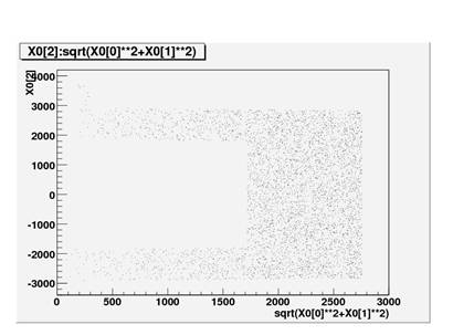
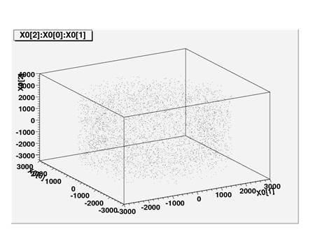
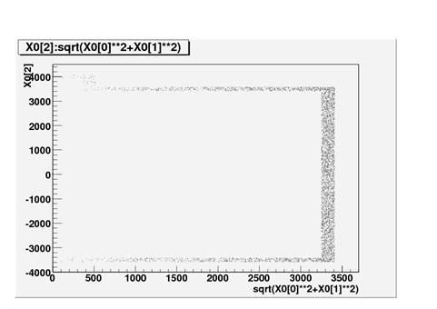
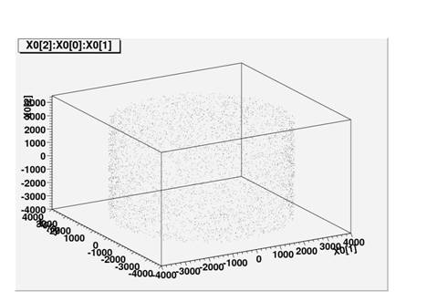
Finally, I obtained a detailed schematic of Double Chooz, and entered an exact coordinate point that lies in the steel of the Inner Veto Shielding Wall. Then I told the macro to fill the steel, and it worked! This happened Tuesday, and for the rest of the week I mainly worked on my final presentation.

Below is a histogram of where I filled the parent events. This looks exactly like the steel shielding on the inner veto wall. These are very, very good pictures.

Week 10: 7/28-8/1

I spent time packing and preparing for my trip to Japan! Also, I’ve been working like crazy to write a program to find the attenuation in the PMT’s. So far, I’ve modeled the PMT’s as a sphere and a cylinder. I realized that the coordinate for each PMT indicates the center of the base of the PMT (the bottom of the cylinder). I also realized that all of the PMT’s point towards the origin. This means that my PMT coordinate is really the normal vector to the plane in which the base of the cylinder lies. Also, the center of the sphere lies along this vector, as does the axis of the cylinder. I’ve been writing code to evaluate whether a given point lies within an area for a given PMT. So far it’s been pretty difficult, and I’m not sure I’ll get it done before I have to leave for Japan. I have almost all of the code written, but I do have to alter some of my lengths that were incorrect, and I also need to change my function that determines whether my point is in the sphere. The PMT’s are more like ellipsoids, so I need to change some of my equations there as well.