August 3, 2006: I had a lot more finishing up work than I thought I did. I've made some pretty sizeable changes to my final report - which is now up and running on the Final Report page - and made a PowerPoint show for the final presentation I will give tomorrow. I will be presenting a 15 minute overview of my project to the other REU students, their advisors, other K-State faculty, my fiancé, and anyone else who cares to come. I practiced the presentation for my group yesterday and made some changes for tomorrow, but I think now I'm all set. I've also been updating my web page to go into its final form since I won't be able to modify it once I leave K-State.
July 27, 2006: Believe it or not, until someone proofreads my report and tells me things they think I should change, my spectrometer characterization is really, absolutely done! That's right, start dancing around in celebration! I know I am!! The whole report is 19 pages long, counting a cover page for the National Science Foundation. Since I'm sure you are just as excited about the whole thing as I am, you can download the entire thing in PDF format from the Final Report page, just as soon as someone helps me convert the whole thing to a PDF file. Until then, try to ignore your ever-growing sense of anticipation and enjoy looking at some of the other stuff on the web site. The data sorting for my group's NH3+ experiment is kind of an ongoing thing, but I'll be spending the rest of my time here at K-State putting as big a dent in that mass of work as I can. Our beamline construction is also on pause for the moment. With any luck, I'll be able to help finish Phase 2 of the epic undertaking. In other excitement, my research group is going out to the Golden Wok tonight for a goodbye party for all the group members (three counting me, although the other two have been at K-State much longer) who are moving on to new physics experiences
July 21, 2006: Still working on my spectrometer analysis. Right now I'm looking at the magnification that the electric charges on the spectrometer plates cause. The electric charges create a field that is curved on the end of the spectrometer, so it ends up acting like a lens, just like on your everyday pair of glasses. It causes a particle that is heading pretty close to the center of the detector in our spectrometer to veer off course and go a lot farther away from the detector (we would say it "magnifies" the y position). We can correct for this in our experiments if we have an equation that says how far off course the particle will go. What I have been doing this week is finding those equations for different conditions in the spectrometer. There two different things that cause magnification: a particle that starts somewhere that is not right in the center of the spectrometer, and a particle that already has some energy that sends it flying away from the center of the spectrometer. There are also two different ways to use the spectrometer: focusing mode (see July 5) and nonfocusing mode. This means that my goal is four reliable equations. I find the equations from the four nifty graphs I'm going to stick below for you to look at. It is a lot of work getting to those nice, friendly looking graphs, but once I do I usually only have to use a fit function on the program that finds all the numbers in their equations for me. I guess I'll put the equations on there too, just because they look delightfully complicated. The Escl is determined by the voltage that is on the spectrometer's main plate and the energy of the particles we are flying into the detector.
These two pictures are for the Nonfocusing Spectrometer:
Magnification of Y position = 1.17901 + 0.71252e -Escl/ 0.29618 + 0.91658e -Escl/ 1.7692 Magnification of Y velocity = 1.02777 + 0.14667e -Escl/ 0.35555 + 0.14628e -Escl/ 1.72715
These two pictures are for the focusing spectrometer:
Magnification of the Y velocity = 0.99362 + 0.0908e-Escl/ 6.23221 + 0.14413e-Escl/ 0.81316
Magnification of Y position
= 0.12996*[e-2 * 2.34253*(Escl – 0.39072) – 2e-0.29636
* (Escl – 0.39072)] + 1.0552 <= This one was particularly
nasty because the program didn't have an equation that would fit the curve, so I
got to learn how to program an equation into the computer. That was pretty
fun. Once we find it from the equation, we just take what physics says a
particle's final position on the detector should be times the magnification, and
that gives us where the particle actually ends up.
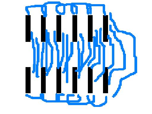
Here's a picture of the electric field lines in the spectrometer, so you can see what the "lens" looks like:
This isn't actually my spectrometer, but it is close, especially for an MS Paint drawing. The blue lines show the electric field. If you look at the middle of the right side, you can see how the field lines curve. That means that charged particles that travel through that field act just like light would when it travels through a glass lens.
July 12, 2006: Whoo! I'm done with the first half of my spectrometer analysis. Boy is that ever exciting. Next I get to look at particles that are already moving when they are in my spectrometer, instead of the nice, optimistic, not-at-all-close to real life situation where they patiently sit still until I tell them they can start flying. I'm currently so incredibly proud of getting the first half done that I might even stick the whole summary on here, if I can figure out how. I did it! Click Here to see my spectrometer analysis in all its half-way-done glory.
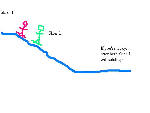
July 5, 2006 Still some really interesting things with characterizing my spectrometer. I'm trying to find the best voltage to use to get space and time focusing. To focus the spectrometer, we have the usual voltage applied to the main plate (plate 5 in the picture below) plus a special focusing voltage on plate 11. The second voltage allows any particles that are lagging behind or flying off center to catch up and get back on track (it acts like the hill in the skiers example below). Since we want to be able to use the spectrometer at whatever voltage sparks the experimentalist's fancy, I think about the focusing voltage as a percent of the spectrometer voltage and use my handy-dandy SIMION program to try different percentages until I find the one that works best. I've got the time focusing pretty well figured out, and I'll be starting the space focusing tomorrow.
Here's a picture of the inside of my spectrometer, minus a detector a long ways away. The graph shows my time focusing data. The title "Error" on the graph means how much time is between the particles when they hit the detector - remember, if it worked perfectly the particles should all get there at the same time. But the best kept secret in the world of physics is Nothing Ever Works Perfectly - hence the need to talk about error. The big blue line is there to show that even though 82.75% gives the best time focusing, any percentage that has an error under 1 x 10-13 seconds (that's where the blue line is) will work pretty well, because our detector only detects particles that are more than 5 x 10-14 seconds or more apart. Then, when I figure out space focusing, we will use the focusing voltage that gives the best overall focusing of both elements, even though it might not be the very best voltage for either time or space focusing.
June 23, 2006: I've spent a lot of this week working on characterizing the spectrometer. Here is one interesting graph. It shows that we need to use a couple tricks called time and space focusing with our spectrometer, because if we don't, two particles with different momentum and starting positions can take the same time to get to our detector.
For all those winter sports enthusiasts out there, you can think about it like two different skiers. If one starts higher than the other, even though the one in front has shorter to go, sooner or later the one in back who is traveling faster (with more momentum) will catch up to the first one. At the point when they are tied with each other, we would say they have the same "time of flight" (TOF).
Up to now (June 22, 2006): I've finished a summary of the first part of my spectrometer characterization, built lots of beamline, just finished learning how to use a computer program to sort the data for the NH3+ experiment, and completed my nifty final shop project so I can use all the tools in our machine shop should it prove necessary. Eventually I'll put a picture of my shop project on here and see if I can talk Mat into showing me how to get one of our NH3 graphs into a file I can put on here, as well.