Class 0x0D: Confidence regions
What is a confidence region?
Given a parameter or parameters fit to data according to a model:
- The confidence region is an interval or area around the best fit point which has a certain probability of containing the true value, assuming the model is correct.
- The probability that the confidence region will include (or "cover") the true value is called the coverage. Different authors may also call it the coverage level or the confidence level or the confidence limit or simply CL.
- A confidence region in a single dimension is also called a confidence interval.
- A confidence region is determined from the data according to some procedure.
Examples
- Upper limit:
- "The hard disk failure rate is less than 0.01/year (95%CL)."
- Lower limit:
- "The expected probability of failure is greater than 0.01/mission (95%CL)."
- Two-sided limit:
- "The allowed
 CL is
CL is  ."
."
Multi-dimensional confidence region:
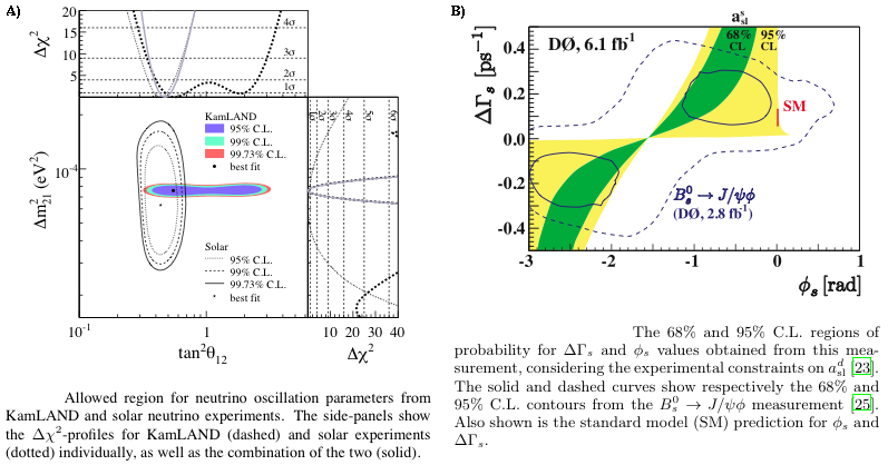
Two-parameter confidence regions for fitted parameters of neutrino oscillations (A) and CP violation (B), taken from [KamLAND2008] and [DZero2010], respectively.
General features of confidence regions
The endpoints of a confidence interval (or the boundaries of a region) are determined by data, and therefore are random variables.
The p.d.f.s of the data in the model hypothesis together with the procedure used to choose the region determine the coverage level.
In general, confidence regions for parameter(s)
 are defined by
where
 is the confidence level. [Larson]
An okay procedure for can have a CL that depends on the true values of the unknown parameter(s) of the model, but still meets the inequality above. A very clever procedure can have a CL that is equal to
regardless of the true model parameter(s).
One such procedure is due to Neyman, described in [PDG-Stat].There are shortcuts for gaussian statistics, and some texts only describe those, but I'll keep it more general.
Desirable features
- A sensible confidence region should ...
- contain the best fit point.
- generally have points inside more consistant the points outside.
- have a known coverage level.
- be consistent and efficient, contracting around the true value as more data is obtained.
- It's possible to come up with procedures that result in regions
without these properties, but that is undesirable.
- Trivial "stupid" example: transform the
 of the data into
a uniform random variable
of the data into
a uniform random variable  . If it is less than 0.1, define an
infinitely thin confidence region; otherwise, define the region to
include all possible parameters. This is an interval, and it has
90% coverage -- but it's not the kind of 90% CL interval we're looking for.
. If it is less than 0.1, define an
infinitely thin confidence region; otherwise, define the region to
include all possible parameters. This is an interval, and it has
90% coverage -- but it's not the kind of 90% CL interval we're looking for.
- Trivial "stupid" example: transform the
Illustration of confidence region coverage
Consider an estimator  for some constant .
Suppose our model tells us that the is a gaussian
random variable with mean and standard deviation
for some constant .
Suppose our model tells us that the is a gaussian
random variable with mean and standard deviation  .
.
What is the difference between the rms of the estimator and the region with 67% coverage?
(Draw picture.)
Confidence intervals are not unique
The following intervals could all have the same coverage and contain the best fit:
How do we choose confidence intervals (Neyman construction)
(Following section 32.3.2.1 in [PDG-Stat].)
Find intervals for each value of the parameter
such that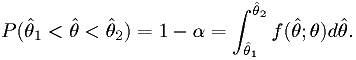
Here
 is the p.d.f. of the estimator .
 and
and  should depend on monotonically.
The functions are invertible:
should depend on monotonically.
The functions are invertible:  implies
  .
.Then (see figure)

Example 1: coin toss
Suppose we toss a coin  times. The coin may or may not be fair. We have
an unknown probability
times. The coin may or may not be fair. We have
an unknown probability  of the coin coming up heads,
  tails.
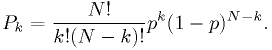
The maxmimum likelihood estimator for is

where  is the number of times the coin came up heads.
The probability distribution of is known:
Example 1a: upper limit
We can find the sum
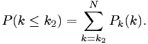
Use that to define the upper limit according to the Neyman procedure. (The lower limit of the interval is set to 0.)
(...picture...)
Example 1b: lower limit
We can find the sum
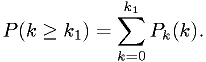
Use that to define the lower limit according to the Neyman procedure. (The lower limit of the interval is set to N.)
(...picture...)
Dangers of one-sided limits
Suppose our procedure (perhaps not consiously decided) were to report
a "95% CL" upper limit for if  turned out very small, and
a "95% CL" lower limit for if the is near 1.
turned out very small, and
a "95% CL" lower limit for if the is near 1.
- E.g., if we got tails all times, we'd report
 at "95%
CL", and do the opposite if we got heads all times.
at "95%
CL", and do the opposite if we got heads all times.
What's wrong with that? Suppose the coin is fair, and  really.
- The 1-sided upper limit excludes this 5% of the time.
- The 1-sided lower limit excludes this 5% of the time.
10% of the time, we make report implying that the fair coin is unfair "with 95% CL".
Example 1c: two-sided limit
One common approach: use  and
and
 to define the intervals.
The only problem is that sometimes this isn't possible. E.g., if we get
tails all times,  , the probability at one end is constrained.
Then we have to adjust somehow,
, the probability at one end is constrained.
Then we have to adjust somehow,
The "unified" method (aka "Feldman-Cousins")
Very similar to the two-sided limit, except we pick the edges of the region to have a given log-likelihood. If the parameter space has a boundary, no problem, just adjust the log-likelihood level to encompass enough space.
In general, the p.d.f. of the log-likelihood is generated via MC for each parameter.
Assignment
Read sections 32.3.2.1 and 32.3.2.2 in [PDG-Stat].
Next Assignment
Build the 90%-CL and 99%-CL confidence regions for the same
exponential + background of the assignment from class 11 (aka class
0x0B), with the restriction that the background parameter  must be
in the range
must be
in the range  and the mean
  must be positive.
- Note this is a good example of where the full Feldman-Cousin's treatment is usually necessary: non-Gaussian model, limits on parameters.
- Just follow the Feldman-Cousins procedure.
| [KamLAND2008] | KamLAND Collaboration, "Precision Measurement of Neutrino Oscillation Parameters with KamLAND", Phys.Rev.Lett.100:221803,2008; arXiv:0801.4589v3 [hep-ex]. |
| [DZero2010] | D0 Collaboration, "Evidence for an anomalous like-sign dimuon charge asymmetry", Submitted to Phys. Rev. D, 2010; Fermilab-Pub-10/114-E; arXiv:1005.2757v1 [hep-ex]. |
| [PDG-Stat] | "Statistics", G. Cowan, in Review of Particle Physics, C. Amsler et al., PL B667, 1 (2008) and 2009 partial update for the 2010 edition ( http://pdg.lbl.gov/2009/reviews/rpp2009-rev-statistics.pdf ). |