Class 0x0C: Hypothesis testing and significance tests
Different cases of hypothesis and significance testing
- Comparison of two hypotheses
 and
and  :
:- The classic "simple hypothesis test".
- Characterized by the significance level of the test.
- Comparison of hypotheses in some model for various values of
some unknown parameters of the model:
- Confidence intervals or confidence regions.
- Characterized by the confidence level of the region.
- Consistency of a single hypotheses
 with data:
- Goodness-of-fit test or significance test.
- Returns a so-called "p-value" which, if small, can be interpreted as the significance of any disagreement.
Simple hypothesis tests
- Test statistic:
- one or more statistic(s)
 , a function of the observations
  .
. - Critical region:
- a region defined by some limits on the test statistic(s).
This is the "rejection region" for .
- Significance level
 of a critical region:
 - Probability for a result to be in critical region if is true.
("Type I error")
- False negative probability
 of a critical region:
 - Probability for a result to be outside critical region if is true.
("Type II error")
 is called the statistical power of the test.
- The critical region is more generally defined as a region in the
full space of measurements . This is equivalent to the definition
here in the extreme case
 .
. - The "reject/accept" terminology is just terminology: "reject "
just means "in the critical region".
- is also called the "null hypothesis". A result outside the
critical region is also called "negative", a result inside is called
"positive". (Think of a medical test where is "healthy",
is a diagnosis of a particular disease.)
- is a probability depending only on the hypothesis
and the critical region, not on any measurements. It is not
a random variable or an observable as such. Similarly, depends
only on and the critical region.
Constructing a good test statistic
We can't simultaneously minimize
and .We can fix
and find the test that minimizes .The Neyman-Pearson lemma says that a test that always achieves the lowest possible
for a given has a critical region
 of the following form:
That is, the critical region is defined by the region where the likelihood of the observation
 assuming hypothesis
is not greater than
assuming hypothesis
is not greater than  times the likelihood assuming hypothesis .
Written another way, the critical region is defined by the test statistic
and the critical region is defined by
 .
.There is a 1-1 mapping between
and . Choose the that
gives the you want. (Obviously, you need to know the p.d.f.s of
both hypotheses to do this.)
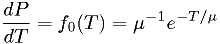
Example 1: unrealistic light bulb models
Suppose we have one model that the p.d.f. for light bulb
lifetime  is given by
for some known  , and another model which is the same except
that the mean is
, and another model which is the same except
that the mean is  , also known.
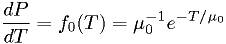
What's the Neyman-Pearson test statistic?
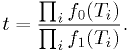
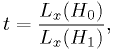
Since we're just going to compare it to a value , we can just as well use
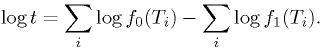
In this case, this is simply

Let's take  . The critical region defined by
  can be rewritten as
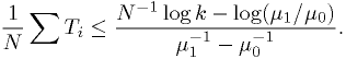
Stated in words: "reject" the larger lifetime hypothesis if the observed
mean is smaller than some amount. Adjust that amount to get the
desired . This can be done assuming a gaussian distribution for
the mean if  is large; otherwise, evaluate it analytically or using
MC methods.
is large; otherwise, evaluate it analytically or using
MC methods.
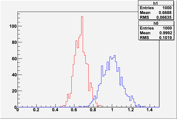
Histograms of the test statistics from example 1
These plots were made with the code in classCh_example1.cc
with  ,
,  , and
, and  .
.
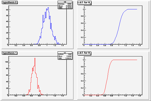
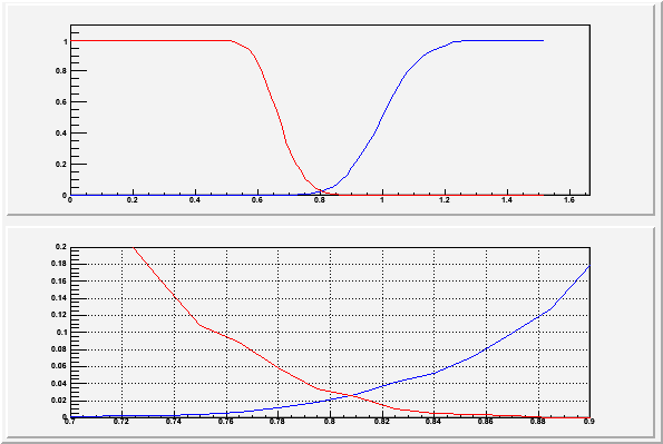
For any given value chosen as the decision criteria on the test
statistic, the value of is given by the c.d.f. of the test
statistic assuming (red curve above), and is given by
1-c.d.f. of the test statistic assume (blue curve above).
Generally one chooses first and then finds the necessary
value of for the decision. The Neyman-Pearson lemma says that
is as low as it can be for that . Note there is in
general no particular advantage to setting  although
there may be reason to do so in some cases.
although
there may be reason to do so in some cases.
Example 2: More realistic light bulb models
Suppose we have one model that the p.d.f. for light bulb
lifetime is given by
for some unknown  , and another model
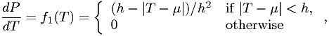
for some unknown and  . Construct the test statistic as
before, and compare the best fit for to the best fit for .
. Construct the test statistic as
before, and compare the best fit for to the best fit for .
Here you might want to evaluate the significance levels for a given
using a MC simulation.
Example 3: applying a signal/background cut
(... see discussion in hypothesis test section of [PDG-Stat] ...)
Two-hypothesis significance test
You don't have to decide in advance at what significance level you will accept or reject a hypothesis.
Depending on what you are doing, it may not even be appropriate to do so. It might be more appropriate to report the significance of the result: the value
 such that the observed data
would be in the critical region for
such that the observed data
would be in the critical region for  ,
out of the critical region of
,
out of the critical region of  .
.For example, you might be investigating a specific alternative to Einstein's theory of general relativity in light of some new data. Rather than report just "hypothesis accepted" or "hypothesis rejected" according to your personal, pre-chosen
, the world would like to know what is. Then
every person can know, for her/his own personal ,
whether they want to accept or reject the null hypothesis.Despite the fact that the significance is often reported as a percentage, it is a random variable. It is definitely not the probability the hypothesis is really right or wrong.
Why the statistical significance isn't the probability you'd like
The significance level,
, is a number you (or someone)
chooses. You adjust your test so it has that probability of giving
you a false positive (type 1 error), on average, over many data sets.- is random variable determined by one measurement or set of
measurements, numerically equal to
 ,
where
,
where  is the value of the test statistic corresponding to the
significance level.
is the value of the test statistic corresponding to the
significance level. What you often most want is
 ,
the probability that the null hypothesis is true given one measurement or
set of measurements. Bayes' theorem tells us
,
the probability that the null hypothesis is true given one measurement or
set of measurements. Bayes' theorem tells us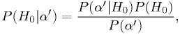
if the truth/falseness of
is itself a random variable.
This might be possible in the case of a medical
diagnosis, but not for a law of nature.- In the case of medicine, we can (perhaps) know all three probabilities
or p.d.f.s for a very well studied diagnostic test:
- the p.d.f. of diagnosis significances for healthy people
 ;
; - the p.d.f. of the diagnosis significance for the
entire population
 , and
, and - the probability of someone in the population being healthy
 .
.
- the p.d.f. of diagnosis significances for healthy people
- In the case of a physical law, we have only one universe to observe,
so this becomes meaningless. Even if we adopt the many universes
idea, we have no way of knowing over the many universes. [*]
- In the case of medicine, we can (perhaps) know all three probabilities
or p.d.f.s for a very well studied diagnostic test:
| [*] | See Comment on Bayesian statistics. |
Goodness-of-fit or one-hypothesis significance test
Again, we have a test statistic, which I'll call .
- The value of should reflect how compatible the data is with the
hypothesis. (E.g., higher values of
 indicate less compatibility.)
 - We should be able to derive the probability
 for any hypothesis.
 - Examples of statistics for which
 is well known include the
for gaussian data and the Kolmogorov-Smirnov statistic for
histogram data. (See discussion in Numerical Recipes [NumRecip].)
is well known include the
for gaussian data and the Kolmogorov-Smirnov statistic for
histogram data. (See discussion in Numerical Recipes [NumRecip].) - The log-likelihood
 is also used, although it requires
derivation or numerical simulation to determine .
is also used, although it requires
derivation or numerical simulation to determine . - As far as I know, there is no equivalent to the Neyman-Pearson
theorem for this kind of test, probably because of the lack of an
alternative hypothesis with which to compare. There's no
universal, general purpose "best approach".
- For example, a test based on
of the measurements might miss an inconsistency that is readily
apparent in a comparison of the histogram of the data points with
the expectation values from the model. (An example of this in
assignment "option B" at the end of this lecture.)
- For example, a test based on
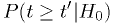
The p-value
The  -value is what the hypothetical model says should be the
probability to find the statistic in a region of equal or lesser
compatibility than the observed : that is,
-value is what the hypothetical model says should be the
probability to find the statistic in a region of equal or lesser
compatibility than the observed : that is,  assuming
is true.
assuming
is true.
- If is in fact true, will be a random variable with uniform
distribution between 0 and 1. [†]
- If is "significantly wrong", then will be a small number.
- The value of
 is often reported as the significance with
which a hypothesis has been rejected. (For an example, see the
claimed rejection of the no-oscillation hypothesis in the abstracts
of KamLAND2004 and KamLAND2002.)
is often reported as the significance with
which a hypothesis has been rejected. (For an example, see the
claimed rejection of the no-oscillation hypothesis in the abstracts
of KamLAND2004 and KamLAND2002.)
| [†] | The proof is the reverse of the derivation of the inverse-distribution-function method of generating a random variable. |
Why this statistical significance isn't the probability you'd like (II)
- The significance of a single-hypothesis significance test is
not the same thing as the signifiance level previously
defined, but it is closely related to the statistical
significance of a two-hypothesis test. Similar comments apply.
- Because is a uniform random variable when is true, if you
reject hypotheses every time they have a -value less than some personal
threshold , you'll eventually end up rejecting a fraction
of whatever true hypotheses you examined.
- You'll also end up rejecting a lot of false hypotheses, but the probability for that will depend on what the true model really is, which this kind of test doesn't consider.
- It's not reasonable to use to select hypotheses to accept, since
can take on any value from 0 to 1 with equal probability when
is true.
Example 4: exponential plus background
How good is the fit of the exponential-plus-background model to the
data in the last assignment? Let's use the best-fit likelihood
 as our test statistic. We'll get the p.d.f. for
using MC simulation.
as our test statistic. We'll get the p.d.f. for
using MC simulation.
:Now just read off the -value from this histogram: according to the
simulation, if the hypothesis is true, what fraction of
would be worse than what you got for the actual data?
Assignment
Choose either "option A" or "option B" below -- you do not have to do both.
- Option A:
- Complete example 4 above.
- Option B:
- See below.
Assignment option B: globular clusters
Are the 119 globular clusters in the Arp 1965 catalog uniformly
distributed in  , where
  is galactic latitude?
- The likelihood of the values is not a good choice in
this case: the hypothesized distribution is uniform,
 doesn't depend on the data values, it's always
 !
! - Instead, try using the likelihood of the values:
 .
. - Make a simple simulation along the lines of the exercise:
- Generate 1000 simulated data sets of 119 clusters distributed uniformly
in
 . Transform to .
 - Accumulate histogram of
 .
.
- Generate 1000 simulated data sets of 119 clusters distributed uniformly
in
- Download the data from Vizier copy of Arp 1965. (Suggestion: download in tab-separated-value format.)
- Read galactic longitude from file, calculate for this
data set.
- What fraction of simulated data sets have less consistent data?
(Lower values of .) If there are almost none, then
the hypothesis can be rejected with some significance.
- Option B' (very optional): instead of (or in addition to) using the likelihood as the goodness-of-fit statistic, try using the Kolmogorov-Smirnov test (see [NumRecip]) or some other test.
Comment on Bayesian statistics
Even though  is meaningless
as a probability in the sense of "the fraction of possible
universes in which would turn out to be true given that
we made these observations", some people like to use Bayes' law
anyway to characterize and update what they call their
"subjective degree of belief". Rather than using objective
data for , they use that term in Bayes' law to reflect
their "prior subjective beliefs" ("priors" for short),
deliberately introducing this as something that can only be
changed by statistically significant evidence to the contrary.
This approach has caused a lot of controversy over the years.
In my opinion, there is nothing wrong with this as long as one
evaluates the resulting p.d.f.s as carefully as possible and
keeps in mind the limitations. However, it can go badly wrong
if the "prior" pre-assigns very low probability to what the
data actually ends up indicating, even if the "prior" is based
on little or no relevant data: for an extreme case, see "The
Logic of Intelligence Failure" by Bruce G. Blair [Blair2004],
actually written by a proponent of this way of thinking. I
won't talk about that further today.
is meaningless
as a probability in the sense of "the fraction of possible
universes in which would turn out to be true given that
we made these observations", some people like to use Bayes' law
anyway to characterize and update what they call their
"subjective degree of belief". Rather than using objective
data for , they use that term in Bayes' law to reflect
their "prior subjective beliefs" ("priors" for short),
deliberately introducing this as something that can only be
changed by statistically significant evidence to the contrary.
This approach has caused a lot of controversy over the years.
In my opinion, there is nothing wrong with this as long as one
evaluates the resulting p.d.f.s as carefully as possible and
keeps in mind the limitations. However, it can go badly wrong
if the "prior" pre-assigns very low probability to what the
data actually ends up indicating, even if the "prior" is based
on little or no relevant data: for an extreme case, see "The
Logic of Intelligence Failure" by Bruce G. Blair [Blair2004],
actually written by a proponent of this way of thinking. I
won't talk about that further today.
References
In the following, (R) indicates a review, (I) indicates an introductory text, and (A) indicates an advanced text.
Probability:
- PDG-Prob:
(R) "Probability", G. Cowan, in Review of Particle Physics, C. Amsler et al., PL B667, 1 (2008) and 2009 partial update for the 2010 edition (http://pdg.lbl.gov).
See also general references cited in PDG-Prob.
Statistics:
- PDG-Stat:
(R) "Statistics", G. Cowan, in Review of Particle Physics, C. Amsler et al., PL B667, 1 (2008) and 2009 partial update for the 2010 edition (http://pdg.lbl.gov).
See also general references cited in PDG-Stat.
- Larson:
- (I) Introduction to Probability Theory and Statistical Inference, 3rd ed., H.J. Larson, Wiley (1982).
- NumRecip:
- (A) Numerical Recipes, W.H. Press, et al., Cambridge University Press (2007).
Other cited works:
- Blair2004:
- B.G. Blair, "The Logic of Intelligence Failure", Forum on Physics and Society Newsletter, April, 2004; http://www.aps.org/units/fps/newsletters/2004/april/article3.html browsed 2010/06/01.
- KamLAND2002:
- KamLAND collaboration, Phys.Rev.Lett.90:021802,2003; arXiv:hep-ex/0212021.
- KamLAND2004:
- KamLAND collaboration, Phys.Rev.Lett.94:081801,2005; arXiv:hep-ex/0406035.