Class 0x0B: Statistics
Quick non-review of probability
I'm going to assume you already know about the following:
- Definition of probability in terms of frequency of occurrence in a large sample.
- Probability density function (p.d.f.) for a continuous variable, and its integral, the cumulative distribution function.
- Joint probabilities.
- Normalization.
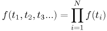
- Definition of independent random variables as having separable joint
p.d.f. (
 iff
iff  and
and  independent.)
 - Bayes' theorem. (
 )
) - Expectation values.
See References.
Example: light bulb lifetime model
Suppose the correct model for the distribution of light bulb lifetimes [*] is
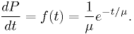
The expectation value for  is the mean,
![E[t] = \int_0^\infty t f(t) dt = \mu](./imgmath/e16601c58979faeada7ca0f12c552267.png)
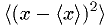
The expectation value for the variance is
![E[(t-\mu)^2] = V[t] = \int_0^\infty (t-\mu)^2 f(t) dt = \mu^2](./imgmath/2d6690db9fdc867e73e6130a62eeac67.png)
| [*] | Note: this is almost certainly not a good model for light bulb lifetimes. |
Caution on probabilities and expectation values
- Probabilities and p.d.f.s are theoretical models.
- They are not observable with perfect precision.
- Given an arbitrarily high number of observations
 , the observed
distributions will converge to the true p.d.f. in the limit
, the observed
distributions will converge to the true p.d.f. in the limit
 .
. - Similarly, expectation values are not statistical means, although
the latter converges to the former in the limit .
What is a statistic?
A statistic is a quantity depending on random variables. A statistic is therefore itself a random variable with its own p.d.f.
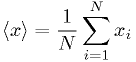
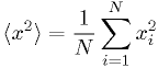
- Examples of statistics on random variables:
Mean:
Mean of squares:
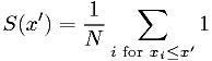
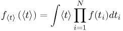
Cumulative distribution statistic:
The last is an example of a statistic that is also a function of a
parameter  . It should approach the cumulative distribution function
as .
. It should approach the cumulative distribution function
as .
Example: statistics of lightbulb lifetimes
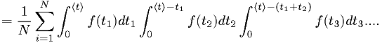
Using the same p.d.f. as in the earlier example, and assuming independent light bulb lifetimes,
- This is not very easy to evaluate.
- However, the central limit theorem tells us that for
 , the
distribution of
, the
distribution of  will approach a gaussian with mean
 ![E[t]](./imgmath/2cad29eb28cc6357b2e0645e5f0378db.png) ,
variance
,
variance ![V[t]/N](./imgmath/ed76c3c74a759c5490cb767003f89e99.png) .
.
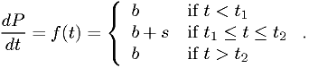
Estimators
- An estimator is a statistic that can be used as an estimate of an
unknown parameter of the p.d.f., such as
 in the example.
 - Statistical moments of the distributions are often useful as estimators.
- Examples:
- Mean:
 can be used directly as an estimator for
 ![E[x]](./imgmath/e7c2a911c6c61006955ae4dd7c35f9c0.png) , since
, since
![E[\<x\>]=E[x]](./imgmath/47923a6dd076e02a6845437e945946d0.png) .
.- Variance:
 provides an estimator for
 ![E[(x-E[x])^2]=V[x]](./imgmath/b9ea7d4f3910091e932f05416747a05a.png) , but
not an unbiased one.
, but
not an unbiased one. ![E[\<(x-\<x\>)^2\>] = V[x]\cdot (N-1)/N](./imgmath/4ff8a24609103e9bd40bb2a8b102f0d6.png) .
.
The statistical moments are not necessarily the least biased, most efficient, or most robust estimators.
Desired properties of estimators
- Consistency (desired perfect):
- Should converge to the correct value as , mathematically.
- Bias (desired low):
- Difference between expectation value and true value, at any .
- Efficiency (desired high):
- Inverse of the ratio of the estimator's variance to the minimum possible variance, given by the Rao-Cramer-Frechet bound.
- Robustness (usually desired high);
- Insensitive to departures from assumptions in the p.d.f. (Somewhat fuzzy.)
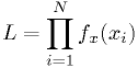
The likelihood statistic
Another statistic one can construct for a data set is the likelihood:
- Again,
 is a random variable, with it's own p.d.f.
 - If the p.d.f.s for depend on some parameters
 , the is also
a function of .
, the is also
a function of . - It is numerically equal to the value of the joint p.d.f. of the
independent observations of .
- N.B. it is not a probability, because it doesn't have the properties
of a probability. In particular, is definitely not a p.d.f. for
or a "probability" of the theory to be true.
Maximum likelihood estimators
- If
 is a random variable, then the value of
that maximizes is a random variable. Call it
is a random variable, then the value of
that maximizes is a random variable. Call it  .
. - is a consistent estimator for .
- It is asymptotically unbiased as .
- Its variance approaches the Rao-Cramer-Frechet bound as ,
i.e., it is efficient.
- may represent any number of parameters.
The variance of maximum likelihood estimators
The inverse
 of the covariance matrix
![V_{ij} = \text{cov}[\hat{\alpha}_i,\hat{\alpha}_j]](./imgmath/5ef4feccea13c1623ce94e71a6d22884.png) can be estimated
using
can be estimated
using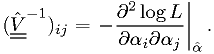
For large samples or perfectly Gaussian probabilities,
has a "Gaussian form",  becomes parabolic in .
- In this limiting case, the
 -standard-deviation error contours
for the parameters
can be found at
-standard-deviation error contours
for the parameters
can be found at 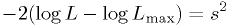 .
.
- In this limiting case, the
Finding proper confidence intervals in the more general case will be discussed in a later class.
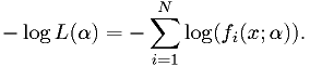
Practical maximum likelihood estimators
It is usually easier to maximize
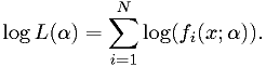
Equivalently, one minimizes the "effective chi-squared" defined as
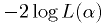 . For Gaussian statistics, this is exactly the
chi-squared, if the standard deviations are known.
. For Gaussian statistics, this is exactly the
chi-squared, if the standard deviations are known.
It is important to include all dependence on in  ,
including normalization factors.
,
including normalization factors.
Example: estimator for exponential distribution
For  ,
,
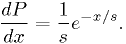
Find the maximum likelihood estimator for .
Example: estimators for double-exponential distribution
For real ,
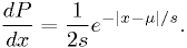
Find the maximum likelihood estimator for and .
Example: estimator for Poisson distribution
For integer  ,
,
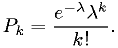
Find the maximum likelihood estimator for  .
.
Example: estimators for Gaussian distribution
For real ,
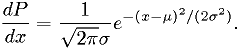
Find the maximum likelihood estimator for and  .
.
Note the estimator for is asymptotically unbiased in the limit
of large , but not unbiased at finite . The bias can be corrected
without degrading the asymptotic RMS of the estimator.
Numerical implementation
Once you know how to minimize a function, and you know the p.d.f.s of the data in your model, then numerical implementation of the maximum likelihood method is easy. Just write the function to calculate:
Then minimize it.
Note: if you have too many parameters, you might need to simplify it some, perhaps by pre-fitting some of the parameters in some faster way.
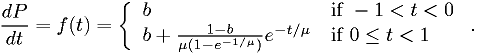
Exercise
Make a maximum likelihood fit of the data in "dataset 1" provided on the course web page to the following model:
By "make a maximum likelihood fit", I mean "estimate the parameters
 using the maximum likelihood method":
- Check normalization of
 .
. - Derive the likelihood function.
- Find an analytic solution.
- Write the function to mimimize into your fitter program and minimize it that way. Compare with analytic solution.
- Plot the solution vs. a histogram of the data and see if it make sense.
Assignment
Make a maximum likelihood fit of the data in "dataset 2" provided on the course web page to the following model:
By "make a maximum likelihood fit", I mean "estimate the parameters
 using the maximum likelihood method":
- Derive the likelihood function. (Turn this in on paper or by e-mailing a PDF or similar document to me.)
- Find an analytic solution (if you can).
- Write the function to mimimize into your fitter program and minimize it that way. (Compare with analytic solution, if you succeeded to derive it.)
- Plot the solution vs. a histogram of the data and see if it make sense.
- Turn in likelihood function, analytic soultion, code, results, and data-fit comparison plot.
References
In the following, (R) indicates a review, (I) indicates an introductory text.
Probability:
- PDG-Stat:
(R) "Probability", G. Cowan, in Review of Particle Physics, C. Amsler et al., PL B667, 1 (2008) and 2009 partial update for the 2010 edition (http://pdg.lbl.gov).
See also general references cited in PDG-Stat.
Statistics:
- Larson:
- (I) Introduction to Probability Theory and Statistical Inference, 3rd ed., H.J. Larson, Wiley (1982).
- PDG-Prob:
(R) "Probability", G. Cowan, in Review of Particle Physics, C. Amsler et al., PL B667, 1 (2008) and 2009 partial update for the 2010 edition (http://pdg.lbl.gov).
See also general references cited in PDG-Prob.