Class 0x0A: Monte Carlo integration and simulation
Simple Monte Carlo integration
Suppose we have some function  of the
  -dimensional
parameter
-dimensional
parameter  . Pick
  random points
  ,
uniformly distributed in volume
,
uniformly distributed in volume  . Then
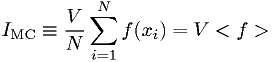
is itself a random number, with mean and standard deviation
![\overline{I_\text{MC}} = \int f dV, \qquad {\large \sigma}_{[I_{\text{MC}}]} = \sqrt{\overline{I_\text{MC}^2}-\overline{I_\text{MC}}^2} \approx \frac{V}{\sqrt{N}} \sqrt{<f^2>-<f>^2}.](./imgmath/a0ca045672f6371560005f2412f631b6.png)
(Here angle brackets are used to denote the mean over the samples, and overline is used to denote the true mean in the limit of infinite statistics.)
In plain English,  is an estimate for the integral.
Integration over many dimensions
- Ordinary numerical integration over dimensions is not easy due to the
number of grid points required,
 if
if  is the number of divisions
on each axis.
is the number of divisions
on each axis. - It often happens that
 fractional accuracy from the MC method
is better than what you can get from the non-MC methods using grid
points with
fractional accuracy from the MC method
is better than what you can get from the non-MC methods using grid
points with  divisions on each axis.
Integration over complicated volumes
If the volume is hard to sample randomly (strange shape),
just define a function that is zero outside the volume and equal to
 inside, and integrate that over an easy-to-sample volume.
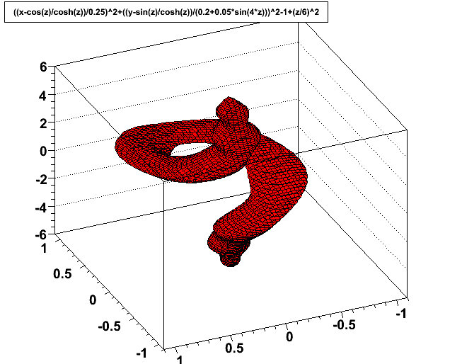
A complicated solid with fine-grained features that would be difficult to integrate analytically or on a numerical grid.
How to get uniform random numbers
Short answer: use a function that returns a (pseudo) random number
uniform in the range  , available from many libraries.
It used to be considered necessary to talk about the pros and cons of various random number generators (RNGs) a great deal, because bad RNGs were commonplace, good ones were hard to find, and computers were so slow it was worth considering using a RNG with poor randomness if it was faster.
The latter two factors are generally no longer true, so a little advice should suffice for the moment.
- Stay away from the standard library function rand(). It tends to be one of the poor ones, for historical reasons.
- The Mersenne Twistor RNG is widely available, and is considered a good choice.
- The Marsaglia-Zaman RNG is also widely available, also a good choice.
- ROOT, CLHEP, and GSL all define various good random number generators for C++, including those mentioned above.
See also: GSL manual section General comments on random numbers.
Example: Mass of an ellipsoidal cloud
The interior of an ellipsoid is defined by
 . Let the density function be
  .
.
 in
in 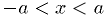 , uniform
  in
in  , uniform
  in
in  :
:Weighting techniques (change of variable)
- If the function being integrated varies strongly on some variable of integration, it helps to redefine the variable to flatten the function.
- This is equivalent to concentrating the distribution of the variable in the more significant region.
Example:
- Let
 in the previous example.
 - Define
 , resulting in
  .
. - Now integrate
 over
over  . The ellipsoidal boundary is
still defined by
. The ellipsoidal boundary is
still defined by  , with calculated from
  .
.
Example: Mass of an ellipsoidal cloud (revisited)
The interior of an ellipsoid is defined by
. Let the density function be
 .
.
 in , uniform in , uniform in
  :
:
Simulation of "unknown" probability distributions
Sometimes you know everything about a random process, except it's too hard to evaluate the resulting probability distribution analytically.
Example: a game of snakes and ladders: you know all the rules, but what is the probability distribution of the number of moves in a game?
One can simulate the process using random numbers and keep track of the distributions of the quantities of interest.
This turns out to be mathematically equivalent to evaluating probability
integrals using the Monte Carlo method, where the dimensions correspond to
all the random variables involved. It may be that is very very large.
Example: Variability of time to sort card deck
If you have a randomly sorted deck of 52 cards, how many steps does it take to sort them using a particular sorting algorithm? Find mean and standard deviation.
Storing distributions in histograms
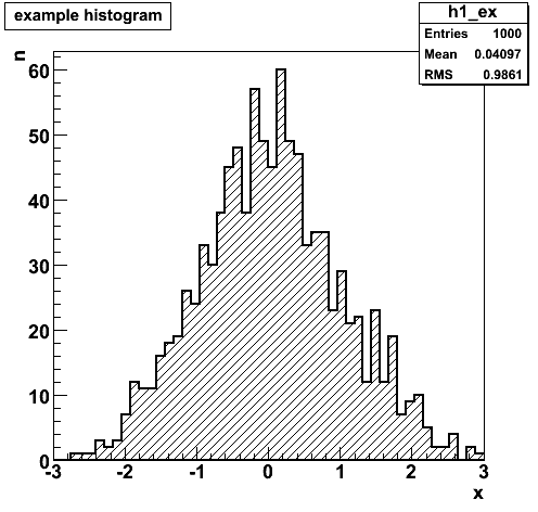
- A histogram is just an array of integers representing a frequency distribution, usually drawn as a bar chart.
- Each integer represents the number of times a particular thing happened.
- For a 1-d histogram of a continuous random number, the "thing that happened" is that the value of the random number fell in a particular range. These ranges are called "bins", and the division of the continuously distributed number into bins is called "binning".
Simple 1-d histogram class
Note: ROOT, GSL, many other packages provide histogram functions, but just to show how easy it is:
class SimpleHisto1 {
 private:
  vector<int> bins;   // stores histogram contents
  double xlow;        // lower end of histogram range
  double xhigh;       // upper end of histogram range

 public:

  // set or reset the histogram range and number of bins
  void Initialize(int nbin, double xlow_, double xhigh_) {
    bins.clear();
    bins.resize(nbin);
    xlow= xlow_;
    xhigh= xhigh_;
  }

  // add 1 to the appropriate bin
  int Fill(double x) {
    if (x<xlow || x>=xhigh)
      return 0;
    int ibin= int( (x-xlow)/(xhigh-xlow)*bins.size() );
    bins[ibin] += 1;
    return 1;
  }

  // get contents of bin i
  int BinContents(int i) {
    return bins[i];
  }
};
Example: time to sort card deck (revisited)
If you have a randomly sorted deck of 52 cards, how many steps does it take to sort them using a particular sorting algorithm? Find the full probability distribution.
Simulation of known random distributions
So far, we've used a RNG which gives a uniform random number  in
the range .
in
the range .
Given such a number , it's easy to get a number that is uniform in [a,b):  .
.
Likewise, it's easy to get an integer  in the range 0..(n-1):
 .
.
And it's easy to get a boolean  with probability
  for true,
 for false:
  .
.
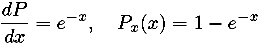
Suppose you need a random number with an exponential probability distribution, or some other distribution?
Inverse distribution function method
Given a uniform random number in the range , we have
Here  is the integral of the probability density, called the
"cumulative distribution function" or simply the "distribution
function". [*] It gives the probability that a given random number will
be less than or equal to a given number.
is the integral of the probability density, called the
"cumulative distribution function" or simply the "distribution
function". [*] It gives the probability that a given random number will
be less than or equal to a given number.
Suppose we want a non-uniform random number , with properties
We can obtain that as follows:
The proof is simple and pleasant, so I leave it as an exercise to the student.
| [*] | Also called the "probability distribution function" in some texts, although this terminology is easily confused with the probability density function (p.d.f.), especially since the density function when drawn actually has the shape of the distribution of the probability. |
Example: exponential distribution
The distribution function for the exponential distribution is easily inverted:
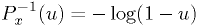
Thus, 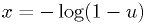 is an exponential random number with the desired
probability density. This can be verified by calculating
is an exponential random number with the desired
probability density. This can be verified by calculating
 .
.
Rejection method
Another way to obtain  , less efficient, is to generate
uniformly in
, less efficient, is to generate
uniformly in 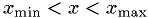 , then generate a second
random number in . If
, then generate a second
random number in . If  , where
  is the largest value can have, then accept , otherwise generate
a new and and try again.
is the largest value can have, then accept , otherwise generate
a new and and try again.
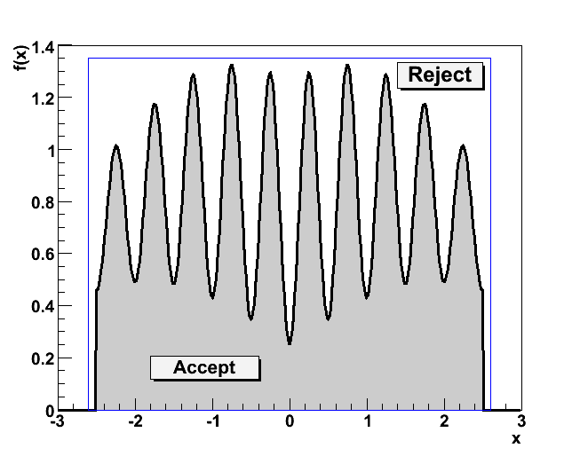
Pairs of  random variables are rejected if outside the
shaded region.
random variables are rejected if outside the
shaded region.
Some pitfalls in using RNGs
- RNGs are really pseudo random numbers. They have a fixed sequence
for a given starting seed.
- Use a different seed if you want different random numbers each time you run your program.
- Use the same seed if you want the same random numbers when you re-run your program (e.g., for debugging a problem).
- RNGs have some number of bits of precision. Be careful not to ask for
more than that.
- E.g., if you have a lousy 16-bit RNG, don't expect it to find events with probability < 2-16 no matter how long you run it.
- Good RNGs have 48 or more bits, but don't try to "take apart" the random number, like if (u<p) { u2= u/p; if (u2<p2) { ... } else { ... } } else { ... }.
Assignment: Random variable resistor network
Suppose I set up 3 variable 1-kohm resistors connected to big knobs in the hallway with a big sign saying "DO NOT ADJUST". Every time a student passes, s/he adjusts the knobs to a random place, uniformly between minimum and maximum. Make the histogram of the total resistor network resistance if one knob is in parallel with two knobs in series, as shown in the figure.
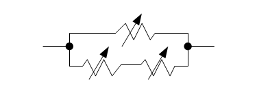
Schematic diagram of the "random knobs".