Class 9: Fitting data

General problem

We have some model with one or more adjustable parameters a_i and a function that describes how well the model fits some set of measurements. Let's call this goodness-of-fit function . This function depends on the parameters of the model, so $F=F(\underline{a})$ .

Our main problem: Find the value of $\underline{a}$ which minimizes . This looks like a job for our function minimizer!

Secondary task: Estimate how far each a_i can be perturbed from its best fit value without increasing the by more than some amount. This is used for estimating parameter uncertainty ranges or tolerances. This can be done using the Hessian matrix at the best fit point.

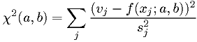
Defining the goodness-of-fit function

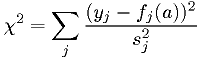
A common choice for the function is the sum of the squares of normalized deviations of the measurements from the model. For independent measurements y_j , and corresponding values from the model $f_j(\underline{a})$ ,

$F(\underline{a}) = \chi^2(\underline{a}) = \sum_j \frac{[y_j-f_j(\underline{a})]^2}{s_j^2}.$

What we choose for s_j depends on our purpose in fitting the model to the data.

When studying what model best describes the data, we set equal to our best estimate of the RMS error of measurement . If the measurement errors are gaussian and independent, we have a true $\chi^2$ random variable.
If we want a function that fits the data for some other purpose, we choose to be appropriate tolerances for that purpose.

There are other possibilities for the goodness-of-fit function. (See Other goodness-of-fit functions.)

Example: voltmeter calibration

Situation: for some reason, you have to use an imperfectly calibrated voltmeter. You record the voltmeter readings at several known voltages from a well-calibrated source. You want to be able to convert any reading to the true voltage. You care more about the accuracy in some voltage ranges than in others.

True voltage	Readout	Readout precision	Required accuracy
0.000	0.000	0.001	<0.001
0.500	0.501	0.001	0.01
1.000	1.006	0.001	0.01
1.500	1.512	0.001	0.003
3.000	3.060	0.001	0.006
5.000	5.139	0.001	0.01
9.000	9.450	0.001	0.01
12.00	12.80	0.01	0.1
18.00	19.80	0.01	0.1

Voltmeter calibration (continued)

Your first idea:: Define the function 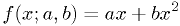, where is the reading, and should give the true voltage. Chose and for best fit of true voltage as a function of readout, using your required accuracy as the weights .
The voltmeter's designer says:: The readout voltage is theoretically a function of the input voltage , with 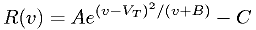$R(v) = A e^{(v-V_T)^2/(v+B)} - C$ , so you should fit readout voltage to true value and invert .

A statistician agrees, and further says you should use the readout precision, not your required accuracy.

What do you do?

Your voltmeter chi-squared function

Go with your first idea:

$\chi^2(a,b) = \sum_j \frac{(v_j-f(x_j; a,b))^2}{s_j^2}$

where x_j is the readout, v_j is the voltage, and s_j is required accuracy. Then you will have your useful and easy-to-use function .

Now just code that $\chi^2$ function and run a general-purpose function minimizer. Start it at a=1, b=0 , which is close to the right solution.

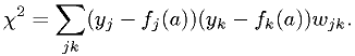
Chi-squared in matrix form

The function

$\chi^2 = \sum_j \frac{(y_j-f_j(a))^2}{s_j^2}$

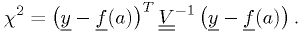
is more generally (in case of correlated measurements)

$\chi^2 = \sum_{jk} (y_j-f_j(a))(y_k-f_k(a)) w_{jk}.$

In matrix form,

$\chi^2 = \left(\underline{y}-\underline{f}(a)\right)^T \underline{\underline{V}}^{-1} \left(\underline{y}-\underline{f}(a)\right).$

Taking the derivatives with respect to $\underline{a}$ and setting them to zero to find the minimum $\chi^2$ ,

$\frac{\partial \chi^2}{\partial \underline{a}} = -2 \left(\underline{y}-\underline{f}(a)\right)^T \underline{\underline{V}}^{-1} \frac{\partial \underline{f}}{\partial \underline{a}} = 0.$

$\underline{f}(a)^T \underline{\underline{V}}^{-1} \underline{\underline{B}} = \underline{y}^T \underline{\underline{V}}^{-1} \underline{\underline{B}}$

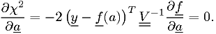
where $\underline{\underline{B}} \equiv [\partial{f_j}/\partial{a_i}]$ .

If we can solve this for $\underline{a}$ , we're done.

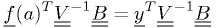
Special case: linear superposition of arbitrary fixed functions

Suppose our model is 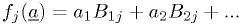$f_j(\underline{a}) = a_1 B_{1j} + a_2 B_{2j} + ...$ , where the 's depend on the measurement index but not on any parameter. In matrix form,

$\underline{f} = \underline{\underline{B}}\ \underline{a},$

where the $\underline{B}$ are fixed. Then general problem for the minimum $\chi^2$ given above becomes simply

$\underline{a}^T \underline{\underline{B}}^T \underline{\underline{V}}^{-1} \underline{\underline{B}} = \underline{y}^T \underline{\underline{V}}^{-1} \underline{\underline{B}},$

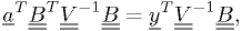
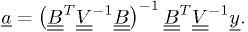
which has the exact solution:

$\underline{a} = \left( \underline{\underline{B}}^T \underline{\underline{V}}^{-1} \underline{\underline{B}} \right) ^{-1} \underline{\underline{B}}^T \underline{\underline{V}}^{-1} \underline{y}.$

Linearizing the non-linear: voltmeter calibration revisited

The voltmeter fit function from the previous example is just the sum of coefficients times fixed functions, exactly the special case above.

So we can solve for the best fit using matrix math directly. (There are many C++ packages that provide classes for linear algebra, including ROOT, GSL, Boost, and others.)
This calculation executes very fast compared to the general function minimization.

N.B. Even though the model for voltmeter was "non-linear", it was a linear superposition of fixed functions. So this is perfect for the "linear fit". This is a commonly occuring case, worth remembering.

Contrast with this case: fit 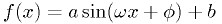$f(x) = a \sin( \omega x + \phi ) + b$ to some measurements y_j for known x_j . The and parameters can be found quickly by the linear fit for given $\omega$ and $\phi$ , but the latter two parameters have to be found by the general minimization routine.

Another example: fitting Bode's law

The mean orbital distance of a planet in the solar system supposedly fits the relation

$a_m \cong A + B \cdot 2^m,$

where $A \simeq 0.4, B \simeq 0.3$ , and

Planet	m	Observed a (AU)
Mercury	$-\infty$	0.39
Venus	0	0.72
Earth	1	1.00
Mars	2	1.52
Ceres	3	2.77
Jupiter	4	5.20
Saturn	5	9.54
Uranus	6	19.2
Neptune	$6\frac{2}{3}$	30.06
Pluto	7	39.44

What are the best and to calculate all planets' mean orbital distances to the same fractional precision?

Assignment: complete fit of Bode's law to planetary data

Feel free to use the minimizer code example from the previous lecture, and just rewrite the function to minimize.

Alternatively, you can base your C++ code on any fitting example from the ROOT website's "howto" or "tutorial" sections.

Alternatively, use the linear fit solution. (But program it, don't just use Matlab or Maple.)

Other goodness-of-fit functions

In other cases, we might use a different function for goodness-of-fit.

Our measurements have non-Gaussian statistics according to our model, and we're really interested in the model or the model parameters themselves:
- Use maximum likelihood method. (Postpone discussion until probability and statistics.)
Our measurements have Gaussian statistics, but there's a correlation between the measurement errors:
- There's a straightforward generalization of the $\chi^2$ function,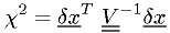
  
  $\chi^2 = \underline{\delta x}^T\ \underline{\underline{V}}^{-1} \underline{\delta x}$
  
  where $\underline{\underline{V}}$ is the covariance matrix. (Derived from the Gaussian probability distribution.)
Our measurements consist of uncorrelated quantities at points:
- Can be treated just like independent measurements.
Our measurements are similar to the previous case, but our model has a large number unknown parameters, each of which affects just the measurements at one of the points:
- Find a fast way to fit each of the parameters at each point (ideally from an analytic analysis, such as the linear fit case). Define the global $\chi^2$ of the remaining parameters, with the parameter already optimized.

There are many other cases, each can be treated by a consideration of the likelihood function and/or the tolerances of your fit for your technical application. Most common cases are covered in the standard references.

References

Press, et al., Numerical Recipes.

G.Cowan, "Statistics", in The Review of Particle Physics, C. Amsler et al. (Particle Data Group), Physics Letters B667, 1 (2008) and 2009 partial update for the 2010 edition. http://pdg.lbl.gov