
Sections
Imagining Light: The Theory of an Interferometer
This Michelson Interferometer is intended to measure the pulse length of the laser coming from the Kansas Light Source (KLS). The idea is that as the laser passes through the interferometer, the beam will be separated then recombined. One half of the beam will be delayed just enough to allow two pulses of the laser to interact with one another. When these two pulses interact they will create areas of constructive and destructive interference and by looking over that interference pattern we will be able to see how long the pulse of the laser really is.
The reason for creating this interferometer was to test the pulse of the laser using an alternate method than the one in the KLS, which uses a Frogger method. The interferometer must also be relatively small so it could be transported to the various experimental sights within the lab. Hopefully the interferometer will not only act as a gauge to find the laser pulse shape but also as a check against the effectiveness of the Frogger.
Imagining Light: The Theory of an Interferometer
The theory of the interferometer is that when you combine two waves you will be able to measure the intensity pattern created by that interference. To measure the intensity of the light its possible to take the absolute value of the square of the Electric field, and when we do this the intensity can be written as:
![]()
![]()
Where
t = time
![]() = the initial
Electric Field and for our convenience we assume that the two electric fields
are approximately equal so it can be factored out.
= the initial
Electric Field and for our convenience we assume that the two electric fields
are approximately equal so it can be factored out.
![]() = distance from
the peak of the wave to the full width half max
= distance from
the peak of the wave to the full width half max
![]() = the time
delay
= the time
delay
![]() = the angular
frequency of the laser light
= the angular
frequency of the laser light
To get the picture of what the intensity is doing as the two pulses pass over one another we integrate this over time t from negative infinity to positive infinity.
We pull the e out of the integral because we assume it to be constant.
Now we have a rather ugly integral which has a combination if trigonometry functions and exponential functions so we convert the cosine functions to their exponential functions leaving us with:

Taking the integrand, expanding it, and then simplifying the square leads us to
This integral can now be broken into three parts and each integrated separately and added together. None of these integrals are easy, but the first two can be found in integral tables and simplify rather easily. The tricky part, at least for me, came in solving the third part of this integral. What is meant in the Real part can be understood using Eulers formula:
![]()
where the real part of this expression is the Cosine function.
Which turns the third part into
![]()
and that can be simplified to
![]()
Now when we evaluate each part of this integral and simplify we find:
What this integral is telling us is that as we change the time delay between the two pulses of the laser they will create an interference pattern that we can measure using a photodiode. Perhaps the integral doesnt say this quite so eloquently but if you listen really closely you can gather its meaning. In listening closely we can see that the only element of either of the oscillating functions that will change with respect to the interferometer is the time delay, so as we change that value the intensity will change. To get a better picture of whats going on we need to take a look at how the interferometer is set up.
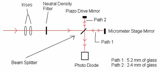
The Michelson Interferometer relies on the fact that light waves will interfere with one another if they are lined up correctly, and because the laser we are working with is indeed light we can get away with this. The way to do this is to send a single beam of light into the interferometer, then split the beam and send it down two different paths that are very nearly the same length, then reflect those beams back through the beam splitter to recombine it and then look at what comes out the other side. To make sure that those two path lengths are nearly the same, or exactly the same as we hope to set it up, we use a mirror that is mounted on a movable stage. The stage can be moved forward and back very precisely, on the order of 40*10^-6 meters (micrometers), to try to match the distance of the two paths very closely. But because we are want the two paths to be exactly the same we added a second mirror attached to a Piezo Drive. The Piezo Drive moves the mirror forward and backward at even smaller increments then the micrometer stage (1*10^-6 m), allowing us to fine tune the difference between the two paths. Then, to ensure that we do not overload our photodiode we insert a neutral density filter which regulates how much light reaches our set up.
Now the question of why comes up. Why do we need to vary the distances that the laser will travel? As I mentioned before we want to make the laser interfere with itself, but what that means is something much more important.
When we delay the laser what is really happening is that we are delaying pulses of the laser so perhaps one pulse is in front of the other like this: compensating plate
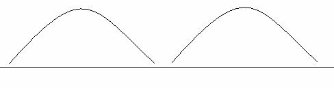
These two pluses are separated by some time and dont interact with one another, so when we look in our photodiode signal or on a viewing screen we wouldnt see anything out of the ordinary. If we decrease the delay between these two pulses then eventually something like this will happen
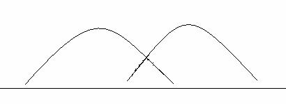
Where the two pulses will begin to overlap and create a small amount of interference. Then if we decrease the difference between the pulses again we can push the two laser pulses on top of each other
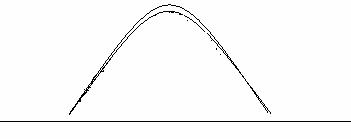
When this happens there will actually be a nearly complete cancellation of the pulses so it will once again look like there is nothing happening, but all around it there will be large areas of interference. The complete overlap of the two pulses leads to what is known as the bulls-eye of the interference pattern. When this happens you know that you are at the exact same distance for both paths.
Changing the path length again and we will eventually run into a situation where the two pulses are only slightly interfering with each other
And finally they will have moved out of range of each other entirely
While this is all interesting unto itself it may not be immediately apparent why we are doing this. Because we have the capability to create and observe interference patterns with our Michelson Interferometer we need a way to apply that to this laser technology. After all, what can a device invented over a hundred years ago do to help us with this cutting-edge twenty-first century laser technology? It just so happens that this is a wonderful tool for measuring the pulse length of our laser.
If you look back to the way the pulses move over one another you can see that one travels a distance relative to the other, but what we are seeing is an interference pattern created by the two pulses interacting with each other. So to figure out how long one of these pulses are all we need to do is keep track of how far we move our Piezo drive from the time we can see an interference pattern to when we cant. I wanted to explain this process in such detail because it is simply so amazing to me that a device created over a century ago for an entirely different purpose could still be helping us today. This truly speaks of the interconnectivity of the physics field. It is impossible to say what sort of technology we will be using ten years from now, so the fact that this piece of technology has lasted over ten times as long is undeniably impressive.
Now that we know what we want to be happening as we make adjustments with our interferometer, its time to take a look at what we can see being delivered to our photodiode.
The photodiode is a very handy tool that measures the amount of energy coming into it and reads it out to an oscilloscope. That is how we can use it to detect the different interference patterns in the laser beam, so when there is a position of high interference we will receive a low signal from our diode and when we reach a region of low interference we can expect a relatively high signal. So with this rational the pictures from before do not do adequate justice to the situation. Instead remember that a pulse of the laser is going to look like a cosine wave formed to a Gaussian curve like this:
The actual laser pulse will look slightly different that this but it will work for our demonstrational purposes.
So imagine two of these pulses as they begin to move over each other. There will be individual parts of the pulse that will contribute to the size of the signal, and then there will be other areas where the waves will cancel each other out. But before we plot what the interferometer should be showing us lets take a look back at what it is were really plotting.
Looking at this integral we can get a good idea of what sort of plot it should make just by applying a few boundary conditions. In this case the variable that we can change in the experiment is L, which is the time delay in the interferometer. First, so we can form a reference point, we should look at the case when L is 0. Our varing functions, the cosine and the exponential, both go to one, and when we look at the case as L goes ether positive or negative we see that that the exponential will continue to decrease until, for all practical purposes, it is zero, but the cosine function will cause the entire expression to oscillate as L changes.
Now when we plug in values for our constants we can get a decent picture of what our interference pattern should look like as we vary the delay distance.
e can be 1 for now because we can treat the electric field of the laser as a constant, t
we will set to be 9*10^-15s or 9 femptoseconds (fs) which is around what we are hoping to find in actual experiment, and w will be set to 2.36*10^15 because we will be using 800nm laser. Graphing the intensity with these values gives us:
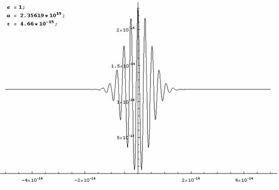
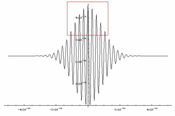
This formula makes it very easy for us to find the pulse length just by looking at the graph of our intensity. If we take the full width at half max of this pulse all we need to do to find the pulse length is count the peaks and then multiply by 2.66 (how far the wave travels in one optical cycle) to find the pulse length.
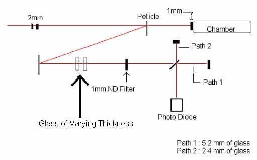
The first time the interferometer was put into action was the week of July 9. Dr. Lew Cocke thought it was a good opportunity for us to see what was happening with the KLS beam that another research team was using. We decided it would be best if we could steel a small percentage of the beam they were using and examine it with our interferometer, and at the same time they could still go about their work because they would still have most of the beam to play with.
To get a small percent of their beam we used a pellicle that was only a few microns thick and placed it in the path of the beam just before it entered their experimental chamber. We then bounced that beam off of a mirror to align it into the interferometer and see if the beam was really like what they were expecting.
As I explained earlier we the way we determined the shape of the pulse was by changing the distance of the delayed path so we would see the entire range of the interference pattern fringes, but we wanted to do this in a way that was controlled and measurable. To do this we hooked the Piezo Drive up to a function generator so we would no longer have to turn the knob by hand and also so it would be a very accurate distance varied over the scan. We then took the signal from the function generator and plugged it into an oscilloscope that would also take in the readings from the photodiode so we could compare the amount of interference with respect to the delay stage (on our graphs the x-axis is the function generator and the y axis represents the photodiode signal).
This is what we were hoping to find:
But this is what we really found:
It turned out that the signal we were receiving from the KLS looked as though it had three main peaks rather than the single Gaussian shape we were expecting. This was particularly unfortunate news for the research team we were borrowing the beam from; this meant that some of their data could be off due to the poor form of this beam.
Despite the irregular shape of the pulse we were receiving we continued with our observations, and we would return to this abnormal pulse shape later to figure out what was causing it.
One of the things we wanted to find out about this pulse was if it was indeed a short pulse as they hoped it would be. So to test this we placed a varying amount of glass in the beam path to see if it would elongate the pulse or not, and perhaps it would change the structure of the pulse that we were seeing without any interference from the glass.
We went about the process by placing different amounts of glass here:
And observing how the interference pattern would change over the scan.
What we were expecting to find was that the pulse would widen after we sent it through more glass. The reason this happens is because different wavelengths of light travel through glass at different speeds, higher frequency light travels slightly faster than lower frequency light. This effect is called chirp. So if we can think of light being broken into different wavelength spectra we can picture whats happening as light passes through glass as the higher frequencies of the light are slightly distancing themselves from the lower frequencies and this will stretch the pulse out. This effect becomes more and more pronounced as the pulse length of the laser become smaller. There are ways to correct for this chirp however. Because we know how the different frequencies pass through material we can use special mirrors to adjust the amount of chirp a laser experiences. These mirrors have several layers which each have different reflective properties. The lower frequencies will be reflected off of the outer surface of the mirror but the higher frequencies will be reflected off of a surface further inside the mirror like this:
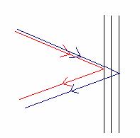
Where the red line indicates the lower frequencies and the blue line represents the higher frequencies.
What these mirrors are effectively doing is moving the lower frequencies of the laser in front of the higher frequencies so when the pulse passes through a piece of glass the higher frequency will have caught up to the lower frequency and the pulse will be lined up again.
What you want is that the frequencies of a pulse to all be in the same spot so knowing how much glass the pulse is going to pass through will allow you to figure out how many chirp mirrors you need to bounce the beam off of so the end result will wined up looking just like it did before the beam passed through any glass. This became very important information for us later in our experiments with the interferometer but for now we were more focused on the result rather than what caused this chirping, and that result was that if the laser was indeed a short pulse we would be able to see an elongation of that pulse when it was passed through an increasing amount of glass.
To get a full spectrum of observations we began with an observation when the laser was under-chirped, that is to say it had more chirping mirrors than it needed for how much glass it was passing through, and to achieve this we simply took out a few millimeters of glass before we took the beam with our pellicle. We then proceeded to add glass by increments of 1mm per trial until we had reached 8mm of added glass to our system.
This is the spectrum with 1mm of glass taken out of the system:

There still seems to be a bit of a triple peak structure

By counting the fringes in this graph we can see that each of the peaks are around the 10fs range which is encouraging even if it isnt in the exact form we would like to see.
This is once again the spectrum when the beam should have no chirp on it at all:

This is the beam with 3mm of glass added:
Now with 6mm of glass added:
And finally 8mm of glass added:
In this last graph the intensity is quite low and we attribute that to the fact that it is passing through so much glass that it is an unavoidable side effect.
Throughout the experiment one can see the continued three peak structure of our observed pulse. This seemed extremely odd to me but Dr. Cocke informed me that they had seen data from other experiments that could be explained by this peculiar triple peak structure of the pulse, so this phenomenon was not unique to our interferometer.
Now I think it is a good time to refresh the fact that what we were seeing with our interferometer is not the pulse itself, but rather the interference pattern from splitting the beam in half and then recombining it; so this triple peak structure is does not mean that the pulse itself has this shape. So now what we needed to find out is what shape of a pulse could cause an interference pattern like this. To figure this out requires a bit of logical deduction that Sherlock would be proud of.
Remember that when two pulses interfere with one another we see a varying amount of interference so if the pulse itself were to have these three peaks we wouldnt see three different peaks of interference, rather we would see five different peaks because one pulse would have to travel across the second pulse and just looking at the first peak of that peak it would interfere three times (the three peaks on the second pulse) plus two more (the two remaining peaks interfering with the second pulse). A good illustration for this is to hold up three fingers on each hand and have these represent a peak, then move these peaks across each other and count how many times any one of these peaks overlaps with a peak on your other hand.
Using this same line of thought we can deduce how to make an interference pattern with three peaks. To have three peaks we need three areas of interference, so when we are looking at the number of peaks on each hand all we need to do is configure them in such a way that they overlap a total of three times. There are plenty of ways to do this with your hand, but remember this is only a convenient way to think about it, the laser pulses are identical so the only way to combine two identical pulses in such a way to make the interference pattern that we see is to have a double peaked pulse. Now going back to our trusty hands we can see that this logic follows. If we have two peaks in our pulses we can make an interference pattern that has three peaks.
Now that weve concluded that it is a double pulse causing the anomaly in our experiment we need to find out where it came from, and if it is indeed from the KLS then we may have uncovered something very important for the efficiency of all of the other experiments in the JRM. Though this would be a very exciting little discovery it would also be a very bad piece of news for all of the research groups that have been depending on the accuracy of the KLS for their experiments which shows that sometimes the biggest discoveries are some of the worst that can be made.
The easiest way to show that the KLS is not at fault would be to show that there is something wrong in our experiment, and in this case being as we have really no authority to go into the KLS and tinker with their equipment and optical setup it is also the smartest way to proceed. So what we needed to do was look at our experiment and see if there was any way that a double pulse could be produced or perhaps taint our results in some way.
One of the luxuries of working with a Michelson Interferometer is that it is a relatively simple machine and does not take a great deal of trouble shooting to see if something is amiss. For one, we do not have many areas where a double pulse could be created in the main mechanism of the interferometer. We did, however, have a case of double reflection in our interferometer when we were working on calibrating the interferometer. In that case we had a reflection coming off of our neutral density filter from the part of the beam that is not reflected to our photodiode. We had addressed this issue at the time but upon inspection the neutral density filter was not the perpetrator of this double pulse.
This was good because at least we knew that the error, if there was one, was not being produced within the interferometer.
Before we had determined the absolute cause of this weird interference pattern I was asked to give a report at Nuts and Bolts on July 16. Nuts and Bolts is a weekly checkup meeting for everyone working in the JRM lab where issues of safety and maintenance can be brought up; it also serves as a time to talk about scheduling for the KLS beam-time and for updates on experiments going on in the lab. On July 16th I stood up and gave the members of the JRM lab the news that there may be something wrong with the KLS, showing them what we had found and that we thought the laser was possibly double pulsing somehow.
After the meeting I spoke with a few members of the research team working directly with the KLS and they suggested that the possibility of having a pellicle in the experiment was the root of our problem, not the KLS. They suggested that if we were using a super thin pellicle, as we were (almost only 10 microns thick), then perhaps we were getting a reflection from the front side of the pellicle and then a second reflection coming from the opposite side of the pellicle. And because this pellicle is so thin it could act as a delay stage short enough to bring two pulses close enough together to make it appear as though it was a single pulse with two peaks.

This suggestion was easy for us to test. We could simply use a regular optical mirror so that we were dealing with the whole beam and thus eliminating the second pulse all together or we could use a thicker pellicle, such as a microscope slide or the like, which would give a large enough delay on the second pulse that it would not interfere with our experiment. If this were indeed the source if the three peak interference pattern then it would be good news for the everyone, especially the KLS.
Before we could do that, however, we had to pick up shop and move to the new experimental site in the lab. This was also an important test of our interferometer because one of the reasons I was instructed to build this device was to have the capability to move from experiment to experiment and test the laser at each site. Written out, or perhaps speaking to someone, this process sounds as though it should be extremely simple; pick up the interferometer from where ever you are, walk to the new spot, put down the interferometer and enjoy. But as anyone who has worked with delicate optical systems knows, and especially when you have to overlap beams of a laser, it is difficult to keep everything lined up. This is true for the interferometer but there was more to be considered.
The Piezo Drive being used on the interferometer was attached in such a way that a mirror was hanging off of it. To understand the problem with this way of doing things I need to say a little something about the inner workings of the Piezo Drive.
The Piezo Drive is able to make such small changes in distance because it is made of a crystal that expands when a voltage is passed across it. This causes the crystal to expand linearly with a very large force (up to 1000 N), but the crystal is only that strong in one direction. If a force is applied on the end perpendicular to the direction it can push it is extremely brittle. So brittle that having a mirror attached to the end of it and walking could potentially break it just from the change of motion involved in taking a step. This meant that while the interferometer was mobile it had to be transported with great care so to not break the part that makes it possible for us to scan over the interference pattern and determine the length of the pulse.
Thankfully we completed the transfer without any problem and the only thing we needed to worry about was making sure that the optics were all in order when we arrived at the second site. We had to make a few minor adjustments but we were able to find the white light fringes much faster than when I had originally put the interferometer together, and in no time at all we were ready to start taking data again.
In the second experimental site that we would be working in we decided that we should heed the advice of the people in the KLS and stop using the thin pellicle and replaced it with a normal mirror. It also was deemed necessary that we needed to adjust the difference in glass that we had in our interferometer. Now that we were fine tuning the interferometer we needed to address the fact that the laser was not passing through an equal amount of glass through the interferometer.
The paths were imbalanced because as the laser hit the beam splitter part was sent through, but a part was reflected off the surface. Then when the beam returned to the beam splitter to be recombined, part of it had to pass through the glass again to reach the recombination point while the other did not have to pass through any glass at all. Finally once the two parts had been recombined they both passed through a section of glass before reaching the photodiode.

This is another problem that is easily corrected; all that needs to be done is to place a piece of glass between the beam splitter and the Piezo Drive that is equal to the difference of glass between the two paths. In this case it is a 1mm piece of glass at a 45 degree angle which is 1.4mm and because the beam to the micrometer passes through this glass twice we need to add a piece of compensating glass that is 2.8mm thick. To add that into the interferometer all we needed to do was add it somewhere on the breadboard, unfortunately we had no room to do something like that. The breadboard was only
12x 6 inches and all of the available space was being used up. This meant that we would have to do a bit of rearranging. With the help of one of the students in the KLS, who was very knowledgeable on the subject, we adopted this layout:

We have a camera mounted on the board as well so that we can see the interference fringes on a display screen when it is no longer visible to the naked eye.
After we had set up this second version of the interferometer we measured to make sure that we had exactly the same amount of glass in our beam path as would be in the experiment that we were taking the beam from. This way we can get as realistic of a pulse as possible. We went so far as to measure out how much air the beam would pass through to reach the experiment and matched the distance for our interferometer as closely as we could.
When we took the data for our second experiment with the interferometer we discovered a rather interesting result.
Running the interferometer this time showed that eliminated that peculiar three peak structure that haunted us in our first try, but now appearing in the data was a strange gap right in the middle of the pulse giving it a saber tooth look about it. Another noteworthy point is that this graph shows more data than we really took, one sweep of the Piezo Drive is indicated here by the vertical red lines. Before we could go into thinking about what was causing this strange shape we went through the same procedure of checking how the length of the pulse varied as we added more glass.
This is a graph of when we had added 0.3mm of glass making the total amount of glass in the system 6.5mm. Once again there is the saber tooth effect in the middle of the data and then two outlying interference patterns. When we continued to add glass up to 2mm thick we saw:
2mm of glass gives us a nearly identical pulse profile as when we were only dealing with 1mm of glass. Finally we worked our way up to 3.5mm of extra glass bringing the total amount of glass up to 9.7mm.
So throughout our data we continued to see this saber tooth in the middle of the pulse, as well as two areas of interference around the large peak in the middle, but overall the peak pattern only became a bit wider. With that in mind we could tell that we were working with a relatively long pulse from our laser, but that still did not explain the odd shape we were receiving, for that we had to step back and look at the big picture for this experiment.
From the structure of the interference pattern we could see a few important things. First: there was something near the middle of the pulse that was causing the two waves to add rather than cancel and second: the pattern for interference indicated that we were not getting a uniform Gaussian pulse shape because we were not getting a Gaussian for our interference pattern.
The solution to these mysteries came from a stroke of genius from Dr. Cocke. He suggested that the pulse was being perturbed by the large amount of chirp correction it was being put through.
The beam was passing through several chirp mirrors and at least half a dozen millimeters of glass. This caused the pulse envelope to shift from being a Gaussian shape to something more like this:
Having a pulse shaped like this suggested that when the two overlap there would at first be an area of small interference:
Then the two large peaks would coincide and create an area of strong interference:
This does not account for the large spike we see in the middle of the saber tooth but I will get to that in a moment, first we can look at the case when the first pulse passes just beyond the second peak:
showing the third area of interference.
The large spike in the middle of our interference pattern is a bit more complicated to explain.
Its possible that the two pulses are somehow slightly out of phase with one another and just at the middle of the two peaks instead of canceling as one would expect them to, they are combined to add to around twice their original value. If you look at the graphs you can see that these data points are roughly twice as high as the surrounding data points, which gives validity to this theory. It is, however, for now just a theory. It would be possible to create a program to graph the integral I solved at the outset of this problem and make the angular frequency a function of time delay as well. Unfortunately due to time constraints I have had no opportunity to pursue this idea any further than its planning stages.
From all of the data that we have gathered I believe that it is safe to say that the interferometer we constructed will be very helpful in maintaining the integrity of the KLS beam. The system is not a perfect one and if I had time to run one more experiment I would truly like to get a beam that has not been tampered with in any way regarding chirp and examine its properties to see if the pure beam is anywhere close to the theoretical prediction. In all honesty I feel that this is the most important step in validating the existence of this interferometer. If this lab really wants a check for the KLS there needs to be a test of the interferometer independent of any other experiment.