Zeeman effect in Mercury
In this experiment you will observe the “splitting” of energy levels in atomic mercury by an external magnetic field. You will quantitatively measure the g-factors of the 63P levels in mercury. There is a section in Melissinos and Napolitano on the Zeeman effect (pp. 218-228 and 239-243) which you should read.
An electron
executing a circular orbit generates a current which in turn produces a small
magnetic moment, ![]() . By the definition of
. By the definition of ![]() , (a current i enclosing an area A)
it can be shown that, for an orbiting charged particle,
, (a current i enclosing an area A)
it can be shown that, for an orbiting charged particle,
![]()
is the angular momentum. If this orbit is subjected to an external magnetic field perpendicular to the orbit plane, one can show classically that the orbital angular velocity is shifted either up or down by
![]()
depending on the sense of the circulation.
The more
correct quantum-mechanical treatment gives a similar result. The energy associated with the orbit is
shifted by ![]() . Suppose we apply B
along the Z-axis. The energy eigenstates of an orbit characterized by a total angular
momentum of size
. Suppose we apply B
along the Z-axis. The energy eigenstates of an orbit characterized by a total angular
momentum of size ![]() , (
, (![]() is the orbital angular momentum quantum number) will be
those with a z component of angular momentum
is the orbital angular momentum quantum number) will be
those with a z component of angular momentum ![]() where
where ![]() . Thus, the external
magnetic field will “split” the orbit into magnetic substrates with energy
shifts given by
. Thus, the external
magnetic field will “split” the orbit into magnetic substrates with energy
shifts given by
![]() (
(![]() if q=e, the charge on the
electron).
if q=e, the charge on the
electron).
The quantity ![]() is called a Bohr magneton, of size
is called a Bohr magneton, of size ![]() A-m2.
A-m2.
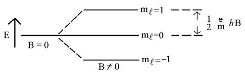
So, for
example, a “2p” level (![]() ) will split into 3 levels:
) will split into 3 levels:
More
complex energy levels for multi-electron systems have both spin and angular
orbital momenta (characterized by quantum numbers S
and L respectively). The total angular
momentum of the system will be the vector sum of orbital and angular momenta. If the
resultant is characterized by total angular momentum quantum number J, the
total angular momentum will have magnitude ![]() with z-component
with z-component ![]() . Now the relationship
between M and
. Now the relationship
between M and ![]() is more complicated:
is more complicated:
![]()
where the factor g depends on L, S and J. It can be shown that
![]()
There are
three strong Hg lines originating from the ![]() (notation
(notation
![]() ) upper level and decaying to the
) upper level and decaying to the ![]() lower levels. These are Green (5460.7
lower levels. These are Green (5460.7![]() , J = 2), blue (4358.3
, J = 2), blue (4358.3![]() , J = 1) and violet (4046.6
, J = 1) and violet (4046.6![]() , J = 0).
, J = 0).
Q: What, for each of these four levels, is L, S, J and g?
A diagram and discussion of the splitting for the J = 2 lower level is given on p. 243 in Melissinos and Napolitano. Read this section.
Q: What should the
splitting look like for J = 1?
J = 0? Draw both the
level diagrams and the expected line pattern for “s” and “p” components (“s” means ![]() ; “p” means
; “p” means ![]() ).
).
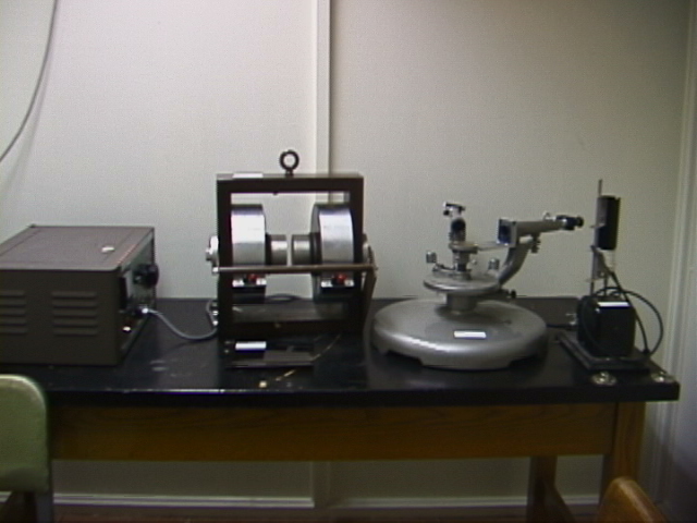
Your apparatus includes:
Hg tube and power supply (5 KV – careful)
Large (al-foil) electromagnet and supply
Prism spectrograph
Fixed separation Fabry-Perot etalon
Polaroid sheet
Hall Probe for measuring magnetic field
TV camera and monitor
Set up the spectrograph with no field so that you can clearly isolate each Hg line. Adjust etalon separately so that the plates are parallel and insert after prism in spectrograph. Tilt it so that you are working off-axis and can see some 10 or so fringes for each line. With no polaroid observe the effect of magnetic field for each line. Do the same with polaroid. You can do this by eye, and also using the TV camera. The TV can see the lines, especially the violet, better than your eye can.
Q: Explain qualitatively the behavior of green, blue and violet lines for each orientation of polaroid. Does the qualitative splitting for each line behave the way you expected it to do?
For your quantitative measurements, take the point of view that your objective is to measure g for both the upper and lower levels. If you start with the violet line, you can use this to measure g for the upper level. Then you can use the blue and violet lines to measure g for the lower level.
In order to do this, you will have to calibrate the splitting you see on the screen of the TV monitor in terms of energy (or equivalently wavelength). You can do this as follows. Suppose you are looking at the fringe pattern for a certain wavelength l. If you had a “knob” on this wavelength such that you could change l slightly, you would see the fringe pattern shift. How much change would it require to make the pattern shift one full fringe? You would have to decrease l enough that where there were n wavelengths between the etalon plates (spaced t apart) of the Fabry Perot before, there would be n + 1 wavelengths instead. The number of wavelengths between the plates is given by n= 2t/ l , so by differentiating this one gets
Dn=- - (2t/ l 2)Dl , or , setting D n=1, the wavelength change needed to shift the pattern by one full fringe is given by
Dl = l2/2t (skip the irritating minus sign: it is not important here).
This calibrates the fringe scale in wavelength. To calibrate this in energy, remember that the energy E of a photon is equal to hc/l, or DE= -(hc/ l2) Dl. From this you can assign an energy scale to the fringe pattern you see. On the TV monitor screen: so and so many eV per mm, for example.
Since the change in the energy of the transition caused by the Zeeman splitting is given by the difference in m dot. B of the upper and lower levels, one arrives at the final result that a change in the energy of the transition DE is related to the magnetic field strength by
DE= m BB D(Mg)
Ideally you would like to measure DE for every line in the Zeeman split spectrum as a function of B. For the violet line, this is easy, since only two lines appear, and each one has a known M upper and M lower. So from this you can use the equation above and your measured DE to find g upper. For the blue and green lines, you will have to work out a puzzle. What DE are you measuring exactly, and how is this related to g lower? From your measured DE values, you can work out an experimental value for g lower , but you will really have to understand what you are looking at to do this. Try to use both s and p lines. Be sure you measure for more than one value of B. See page 242 in Melissinos and Napolitano.