 Analysis of Density of Rb MOT
by Cameron Cook
supervisors:
Brett DePaola, Larry Weaver
Week 2: This week I continued learning
more about the experiment and why these atoms are acting the way to do
concerning their photonic emission.(elaborate more about what I read) We had
safety training for the JRM lab and for the wood and metal workshop. Also, I
designed a simple mount for a new CCD camera to sit on and view into the MOT.
Week 3: Monday I built my camera mount
in the student workshop with supervision. It works and looks great; here’s some pictures. I started some tutorials on the
programming language Python. This will be handy later since I will be
developing a couple programs later in the summer and I have minimum experience
in programming. I’m also reading about BASEX, POP,
and the Iterative method. These programs are inversion techniques that pull 2-D
plots into 3-D density distributions and should help me determine the MOT’s density. They each have their pros and cons.
Week 4: Vince fixed up my computer so that the digital
camera would connect to the computer and so that the image would show in
Labview. The MOT was a little shy in its first photo shoot. Bachana and I had
to find the little guy in the chamber. There was much distance changing,
refocusing, and searching for the MOT. The fluorescence is near infrared, just
outside of human vision, so human eyes can’t see the
MOT, but a CCD filter is capable of sensing it.
Finally
got some decent resolution and size images. Here’s one of
them:
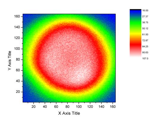
This is an image after
I’ve prettied it in Origin 8. The axes are the number of pixels. 1 millimeter
is equivalent to about 70-80 pixels, so this is pretty huge for atomic
standards. The legend to the right is a measure of the fluorescent intensity.
Notice the dip in intensity in the middle of the graph. Pretty odd- could be
destructive interference of the light, maybe it’s so dense that the outer atoms
are absorbing some light that the inner are emitting, or there could actually
be a dip in the real atom cloud. I think the second option.
Now, run the image
through the BASEX program, and I get this inverted image:
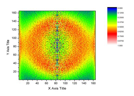
BASEX inverts the image
line by line, and so all the noise in the image is pushed inward, creating the
blue center line. BASEX concurs that there is a dip in density. The center blue
line and the extra red on the left and right sides are artifacts of the
program.
Week
5: This week, with help from Brett, I wrote a Python
code that takes user input of the number of rows and columns of a designated
matrix and it performs an inverse abel transform on the inverted image from
BASEX. The MOT contains a cylindrical symmetry. Because of this, one doesn't
have to worry much about the z axis due to its symmetry throughout. Therefore,
the main concern is summing up all of the pixels in polar coordinates around
the middle origin. From an integral of sqrt(x^2+y^2) for all values of radius,
one will obtain the deconvolution of the inverted image, i.e. the 2-D intensity
plot derived from the 3-d density distribution.
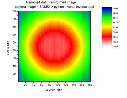
This is
Python’s deconstruction that I made.
Also, the program contains a
subprogram that takes a fractional error between the deconvoluted image and the
raw image from the camera. By subtracting the deconvoluted image plot counts
from the raw image and dividing by the raw, it gives a matrix that plots the
difference between the two programs so that I can see how accurate BASEX is
inverting my images.
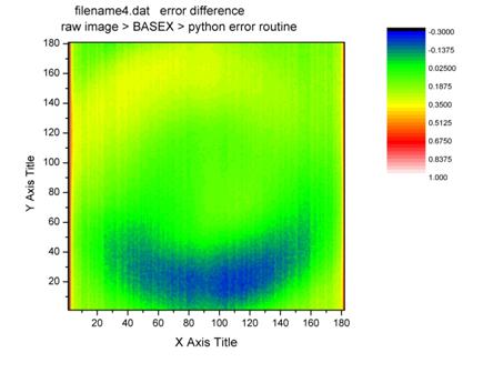
This is the error graph. It shows
a -30% error in the blue area, about 35% error in the yellow, and about 2%-10%
in the middle green.
Doesn't seem ideal.
Week
6: I made
another Python program that takes the deconvoluted images made from the program
I made last week and puts a running average of any value the user decides. One
can input any odd number and the program will put a running average on the
values in the matrix in order to smooth out the deconvoluted image. The thought
was that this running average would produce a more accurate image that is more
similar to the raw image. Its change was negligible.
I measured the spatial
calibration of the camera to the MOT. As the camera was 7 cm from the viewing
glass of the MOT, I took a picture of the MOT chamber without the laser on.
Brett told me the distance between the plates in the chamber. With that
knowledge, I measured the pixel distance and determined the spatial ratio is
about 85 pixels per millimeter.
Week 7: Tested BASEX with fake matrices, and it proved useless to us.
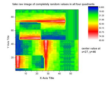
This is the fake
matrix. There is no symmetry between the quadrants.
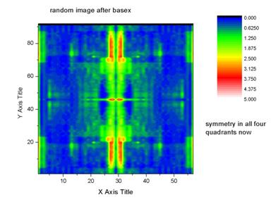
This is the fake matrix
after a run through BASEX. No boxes are checked in the program that would
assign some symmetry to the image, yet there is some type of averaged
superimposed symmetry from all four quadrants. These results are not good for
an original image that is not symmetrical radially, horizontally, nor
vertically.
Now
I am trying to learn the Vrakking code in FORTRAN so that I can adapt it to my
particular data. Vrakking is supposed to not assume any symmetry, is supposed
to be better for unsymmetrical images, and suppose to have less error than
other deconvoluting programs. It is also slower than other programs, but time
is not an important issue to me. It only takes 25 seconds for the program to
run, compared to BASEX's 12 second record.
I
learned it well enough to run the program I got from De Sankar, a postdoc here.
This edition of the Vrakking Iterative method works in a circular manner,
whereas BASEX was line by line. This supposedly makes most of the error
accumulate in the middle. Within the program it creates several files, one that
makes a target image, what the program tries to iterate the image into, a
simulated image, the actual 2-D deconvolution the program makes from the target
image, an inverse image, the 3-D plot, and an error plot. These matrices are in
cartesian coordinates, and the FORTRAN code also makes another set in polar
coordinates. After looking at all of the files, especially the error files, I
decided Vrakking was unsatisfactory.
This
is the raw image again.
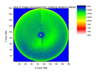
This
is a slice of Vrakking’s inversion.
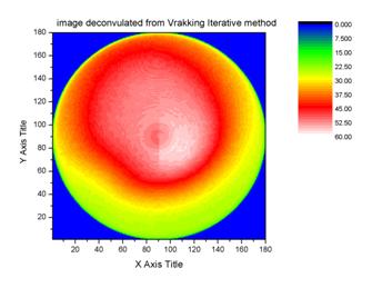
This is
Vrakking’s deconstruction. After creating the deconstruction, Vrakking compares
it to the raw and adjusts itself to improve its deconstruction so that it looks
more like the raw. It repeats the inversion process over and over until the
deconstruction is very close to the raw.
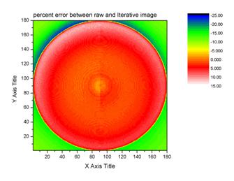
This is
the error graph made from a Vrakking subprogram. This final deconstruction has
an average error of less than 5%, which is good.
This
week was temporal calibration between the laser and camera. In my setup, the
laser first hits a diverging lens. Very far downstream along the laser, the
diverged beam encounters an iris. As the beam's Gaussian shape is diverged, the
iris serves to allow only the centermost part of the beam pass. This cuts off
the maximum of the Gaussian shape and can be approximated as a flat plateau, in
order to assume the same changes are being made to all affected pixels on the
camera. After the iris, there is a neutral density filter of 3 (so it lets only
a thousandth of the intensity of light through; this is so that the camera
doesn't become saturated), and I measure the power with a power meter. After
the attenuator, the camera is situated for prime viewing of the laser.
With
this setup, I took several pictures. One set had a constant gain as I switched
the shutter speed. The next set had constant shutter speed as I altered the
gain. From each graph, I took the value of a certain pixel. I plotted each
respective set with one axis being either gain or shutter speed and the other
being the count value of the pixel. The shutter speed showed a linear graph in
respect to count number. The gain graph
showed an exponential curve with an offset. The graphing program provided me
with these parameter values of the exponential curve.
The
program that is used to take pictures also provides a total sum of the pixel
counts in the picture. One pixel can range from 0 to 255. 255 is the extreme
limit of intensity and the camera is most likely saturated if the counts are
this high. With all of these values at my disposal, I could relate the sum of
the pixel counts, gain value, and shutter speed value, to find a conversion
factor and be able to predict the power of the laser. By knowing the power of
the laser from this, the MOTRIMS group will be able to measure the intensity of
light emitted by the MOT and predict the power that is emitted to the MOT. By
relating power to the rate of photons per second, one may determine how many photons
are being emitted by the MOT. Then, through another relationship of spontaneous
emitted photons to stimulated emitted photons, one may calculate the amount of
stimulated photons and the atomic density of the MOT. (The camera only sees
spontaneous emission because the stimulated emission follows the path of the
laser.)
I
go more into detail on my powerpoint presentation and my poster.
I
also measured the attenuation of the camera lens. It has an attenuation of
.0813.